In previous article, we have introduced you the method to sum if cell is equal to a certain value, you can check “How to Sum Numbers by Formula if Cells Equal to A Certain Value” on our website for reference. By the way, if special characters exist in the target, can we use the same method to sum numbers? In this article, we will show you how to ‘sum if cell contains special character’ by formula with the help of Excel SUMIFS function.

Through demonstrate a simple instance, we will introduce you the syntax, arguments of SUMIFS function, and let you know how the formula works step by step and finally reach your goal. After reading the article, you may have a simple understanding of SUMIFS function. We will also introduce you another method to resolve this issue by SUMIF function at the end.

EXAMPLE

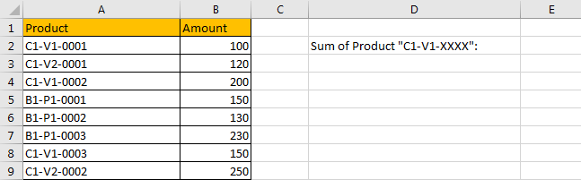
Refer to above table, we can see that some different types of products are listed in “Product” column. Product serial number consists of three parts, and the three parts are connected with special character “-”. Amount for each type product is listed in “Amount” column accordingly.

In this instance, we want to calculate total amount for the product which serial number is combined with “C1-V1-xxxx”. So, only the products which the first two parts are “C1-V1” can meet the condition. We need to find out all proper products, and then sum up values in “Amount” column. To resolve this issue by formula, we can apply SUMIFS or SUMIF functions.

FORMULA – SUMIFS FUNCTION

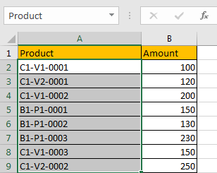
Step 1: Select A2:A9, then in Name Box define a new name for this range, for example ‘Product’.

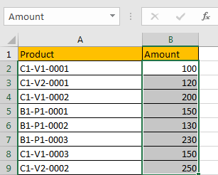
Step 2: Select B2:B9, in Name Box define a new name for this range, for example ‘Amount’.

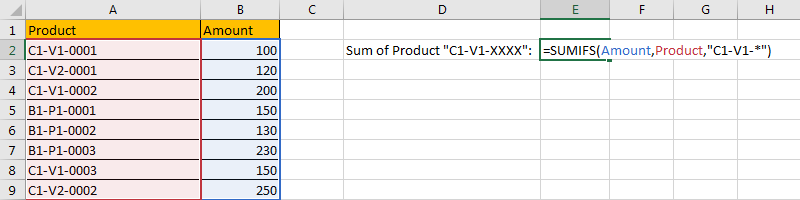
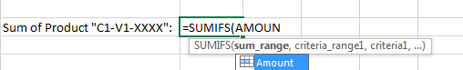
Step 3: In E2, enter the formula =SUMIFS(Amount,Product,”C1-V1-*”).

NOTE: In step#1 and step#2 we defined range name “Product” and “Amount”, when entering the formula, after typing “Amou…”, defined range “Amount” is auto loaded, you can directly select it from dropdown list. You can also select B2:B9, A2:A9 to fill formula arguments as well.

Step 4: Press Enter after typing the formula.

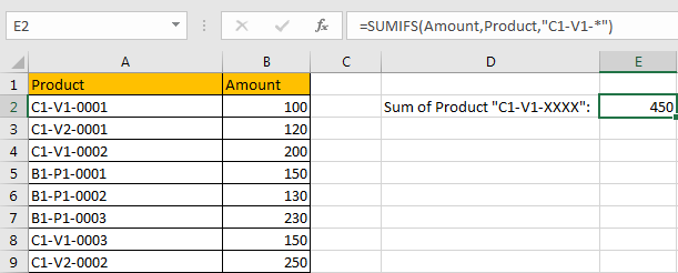
We can see in column A, cell A2, A4 and A8 contain “C1-V1”, the corresponding amounts are 100 (in cell B2), 200 (in cell B4), and 150 (in cell B8), so the total is 100+200+150=450. The formula works correctly.

SUMIFS FUNCTION INTRODUCTION

SUMIFS function can be seen as SUM+IFS, it can handle multiple ‘criteria range’ and ‘criteria’ combinations.

For SUMIFS function, the syntax is:

SUMIFS(sum_range, criteria_range1, criteria1, [criteria_range2, criteria2], …). Contents in [] are optional.

SUMIFS function supports wildcards like asterisk ‘*’ and question mark ‘?’, it also supports logical operators within its arguments. If wildcards or logical operators are required, they should be enclosed into double quotes (““) with text.

The usage of wildcards:

1. An asterisk (*) means one or more characters.
2. A question mark (?) means one character.
3. The position of asterisk or question mark means the character(s) position relative to the entered part. For example, “*A*” means characters or texts are both listed before and after “A”. “A*” means this text is started with A, but ends with others.

The usage of logical operators:

1. “>” – greater than
2. “<” – less than
3. “<>” – not equal to

ALL ARGUMENTS

SUMIFS – SUM RANGE

In our instance, B2:B9 is the ‘sum range’ obviously. Amount values are listed in this field. We define this range with name ‘Amount’ in above step#2.

In the formula bar, select ‘Amount’, press F9, values in this range are listed in an array.

SUMIFS – CRITERIA RANGE 1

A2:A9 is the criteria range. In this instance we have only one criteria range. This range contains different types of products.

In the formula bar, select ‘Product’, press F9, values in this range are listed in an array.

SUMIFS – CRITERIA 1

We want to calculate total amount for the products contain “C1-V1-”. In this criterion a special character “-” exists, as we mentioned above, SUMIFS function supports texts and special character, so just enter “C1-V1-” to fill the criteria. As cells are not ended with “C1-V1-”, the completed combination is “C1-V1-XXXX”, so a “*” is added after “C1-V1-” to represent “XXXX” part. After all, for criteria 1, we enter “C1-V1-*” to fill this argument.

HOW FORMULA WORKS

After explaining each argument in the formula, now we will show you how the formula works with these arguments.

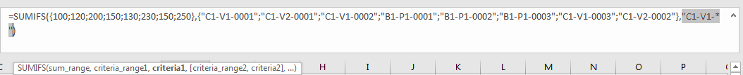
Refer to above mentioned arguments, the formula is converted into below format in the formula bar.

=SUMIFS({100;120;200;150;130;230;150;250},{“C1-V1-0001″;”C1-V2-0001″;”C1-V1-0002″;”B1-P1-0001″;”B1-P1-0002″;”B1-P1-0003″;”C1-V1-0003″;”C1-V2-0002″},”C1-V1-*”)See screenshot below:

See the pair of criteria range and criteria:

Criteria Range 1: {“C1-V1-0001″;”C1-V2-0001″;”C1-V1-0002″;”B1-P1-0001″;”B1-P1-0002″;”B1-P1-0003″;”C1-V1-0003″;”C1-V2-0002”}

Criteria 1: “C1-V1-*”

In criteria range 1, compare each product serial number in the array with “C1-V1-*”; if “C1-V1-” exists in product serial number, mark them in bold:

{“C1-V1-0001“;”C1-V2-0001″;”C1-V1-0002“;”B1-P1-0001″;”B1-P1-0002″;”B1-P1-0003″;”C1-V1-0003“;”C1-V2-0002”}

So, for bold texts, record a ‘True’ in the array; otherwise, record a ‘False’. Then we can get a new array:

Array 1: {True;False;True;False;False;False;True;False}

Convert ‘True’ to ‘1’ and ‘False’ to ‘0’:

Array 1: {1;0;1;0;0;0;1;0}

Now, we have below two arrays:

Sum Range: {100;120;200;150;130;230;150;250}

Array 1: {1;0;1;0;0;0;1;0} – from above steps we know that if cell contains “C1-V1-”, 1 is displayed.

We list the two arrays in two rows, in the same column multiply the two numbers, and save their product in another row.

Sum up all numbers in the third row.

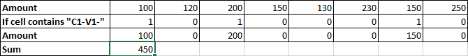
100+200+150=450

COMMENTS

In this case, we can also use SUMIF function to sum cell properly.

For SUMIF function, the syntax is:

=SUMIF (range, criteria, [sum_range]). Argument in [] is optional. If sum range is omitted, SUMIF will sum up all numbers in range argument.

In E2 enter the formula =SUMIF(Product,”C1-V1-*”,Amount).

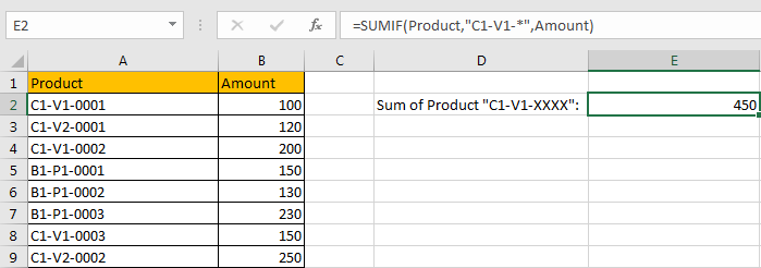
After entering the formula, we can see that SUMIF function also works correctly. Actually, in most situations, SUMIF function can be used instead of SUMIFS function, the difference is SUMIF function can only support one pair of criteria range and criteria. So, if only one criterion is supplied to filter data, you can select either SUMIF or SUMIFS you like to sum cells.

SUMMARY

1. SUMIFS function can handle multiple groups of criteria ranges and criteria. Sum range is the first argument among all arguments.

2. It supports user defined range name.

3. It supports wildcard.

4. It supports logical operators.

Related Functions

---

• Excel SUMIF Function
  The Excel SUMIF function sum the numbers in the range of cells that meet a single criteria that you specify. The syntax of the SUMIF function is as below:=SUMIF (range, criteria, [sum_range])…
• Excel SUMIFS Function
  The Excel SUMIFS function sum the numbers in the range of cells that meet a single or multiple criteria that you specify. The syntax of the SUMIFS function is as below:=SUMIFS (sum_range, criteria_range1, criteria1, [criteria_range2, criteria2], …)…