In daily work, if we sort data with blank cells included in the same column, these blank cells are listed at the bottom automatically after sorting. If we want to keep the positions of these blank cells unchanged and only sort the others, how can we do that? In this article, we will show you the way to sort data in this scenario.

EXAMPLE

          ->         

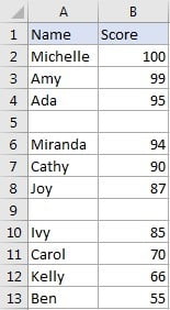
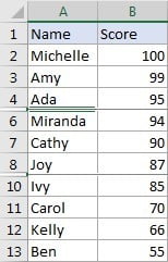
There are two blank rows listed in above table. We want to sort data by score column with the two blank rows locked in row 5 and row 9. Normally, if we select score column and directly click sort “Z to A” button to sort data, the two blank cells are listed at the bottom, this behavior is not our expectation.

In fact, if we want to sort data with blank cells locked in their own positions, we can hide them firstly, then sort data in visible cells. After sorting data by proper order, we can unhide the hidden rows, the blank cells are still listed there.

STEPS

a. Select range A2:B13, then click Home in the ribbon, in Editing section click Find & Select button to see options for finding texts in document.

b. Click Go To Special option.

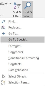
c. In Go To Special dialog, check on “Blanks” option. Options in this dialog are exclusive. Then click OK button.

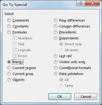
d. After clicking OK, all blank cells are highlighted.

e. Keep blank cells highlighted. Press Ctrl+9 to hide rows. In Excel, Ctrl+9 can hide rows with cell or range highlighted. If you want to unhide rows, you can press Ctrl+Shift+9. If you want to hide columns instead of rows, you can press hotkey Ctrl+0.

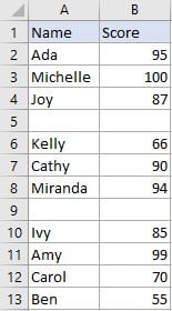
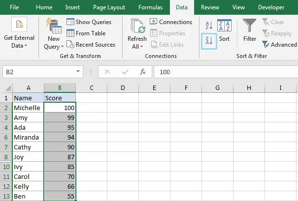
f. Now, select B2:B13 with blank rows hidden, click Data in the ribbon, click Sort Largest to Smallest button in Sort & Filter section to sort numbers in B2:B13 from the largest to smallest.

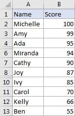
g. After sorting, numbers are sorted from the largest to smallest properly.

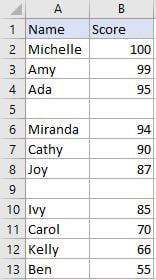
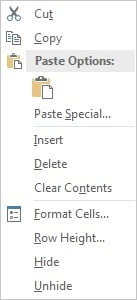
h. Select entire rows from row 2 to row 13, right click to load row editing menu, click Unhide.

Blank cells (rows) are still listed there.