Sometimes we need to merge two tables data from different sheets into one table, for example merge data in sheet2 to sheet1 based on some criteria, how can we do? Except copy data from sheet2 to sheet1 one by one, we have another way to merge data by function VLOOKUP in Excel.
First, prepare two tables. As we all know, Excel is very useful for creating table to record data, and its format is similar with database. As in database there is always a major key in the first column to relate to other tables, so here we can create two tables in two sheets with a common column like database. Be aware that the two sheets must have a common column, then we can merge data based on this column later.
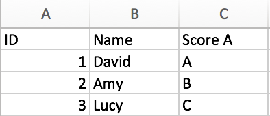
Sheet1
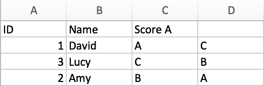
Sheet2
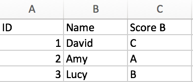
You can see that for one student they have two scores on different sheets, we want to merge them into one table in sheet1 like ID & Name & Score A & Score B. We find they have the same columns ID and Name, we will use ID as the key column to do demonstration. Now let’s follow below steps to start to merge data.
Step 1: In sheet1, D column->cell D2, enter ‘=vlookup’ to call VLOOKUP function.
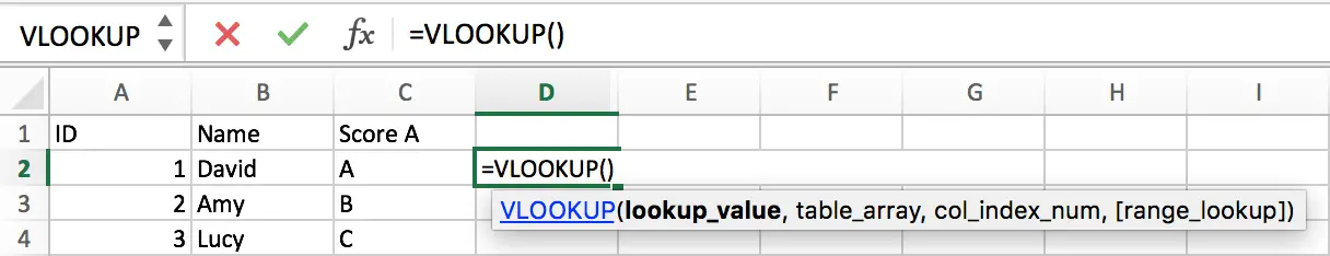
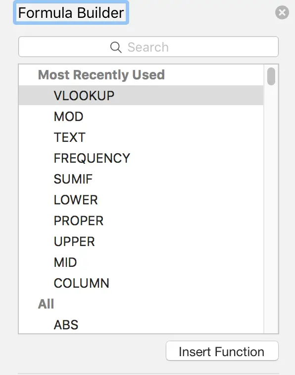
You can also click on Formulas->Insert Function to load Formula Builder to insert VLOOKUP function.
Step 2: Refer to each parameter in VLOOKUP function, enter the actual values and ranges in VLOOKUP function on cell D2.
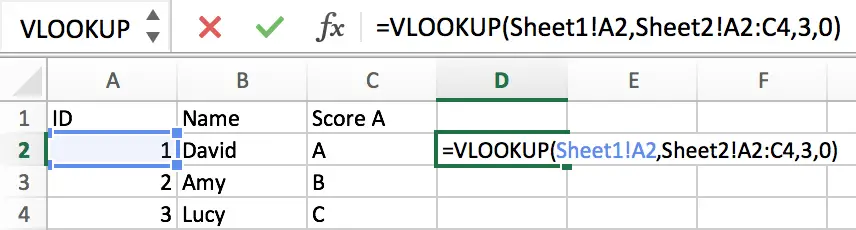
As column A exists in both two sheets, so we can use this column to connect two tables. The Lookup value is cell A2 in sheet1->column A, then search it from range sheet2 ->A2:C4, then returns Score B which is listed in the third column in sheet2, so finally we entered the formula as follows:
=VLOOKUP(Sheet1!A2,Sheet2!A2:C4,3,0)
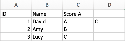
Step 3: Click on Enter in cell D2. Then we get what we expect.
Step 4: Copy cell D2 to D3 and D4. Or drag it down to D4 directly with formula copied.
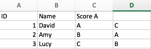
Here we get a complete table with both Score A and Score B now.
Step 5: If we change the ID orders for students in sheet1, and use the same formula to connect data, we will get an Error this time.
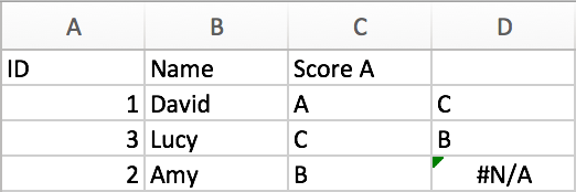
Here we cannot find proper mapping Score B for Amy.
Step 6: Click on cell D2 and D3 to check the formula again.
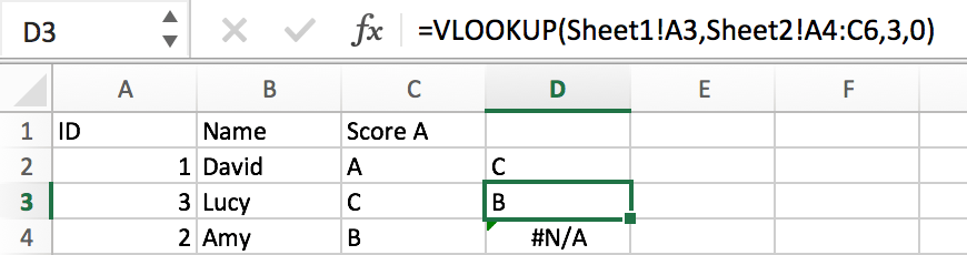

We find that the root cause of this error is the search range from sheet2 is moved from A2:C4 to A4:C6 (A5:C7) improperly. So we need to add $ before the range to make VLOOKUP to search the fixed range absolutely.
Step 7: Re-type formula into cell D2 ‘=VLOOKUP(A2,Sheet2!$A$2:$C$4,3,0)’.
We merge two tables into one properly.
Related Functions
- Excel VLOOKUP function
The Excel VLOOKUP function lookup a value in the first column of the table and return the value in the same row based on index_num position.The syntax of the VLOOKUP function is as below:= VLOOKUP (lookup_value, table_array, column_index_num,[range_lookup])….