This post will guide you how to create graph paper template in your worksheet in Excel. How to do I turn an Worksheet into graph paper in Excel 2013/2016.

Make Graph Paper Template

---

To Make a worksheet as graph paper in Excel, you just need to do the following steps:

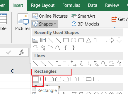
Step1: go to Insert tab in the Excel Ribbon, click on Shapes command under Illustrations group, and then select Rectangle from the Rectangles section.

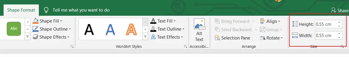
Step2: you can draw a rectangle in your current worksheet, and then you need to go to the Shape Format tab, and specify the rectangle’s height and width in the Size group. you should set the same size for both height and width.

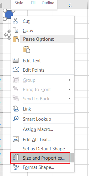
Step3: right click on it and select the Size and Properties from the drop down menu list. And the Format Shape pane will appear.

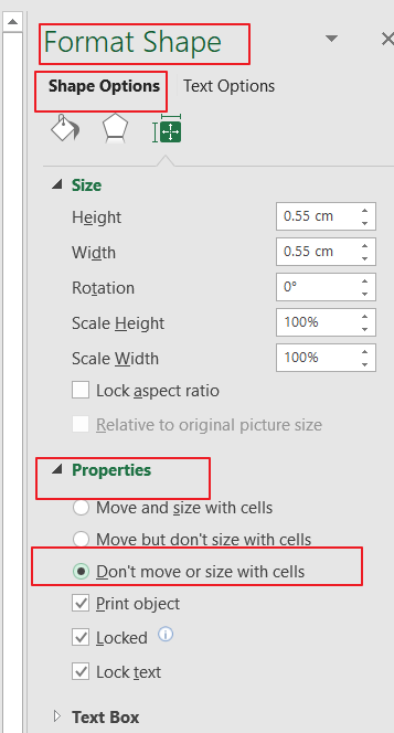
Step4: check the option Don’t move or size with cells option in the SHAPE OPTIONS .

Step5: move the rectangle to the top-left corner, just over Cell A1.

Step6: select any one cell and then press Ctrl + A keys on your keyboard to select the entire worksheet.

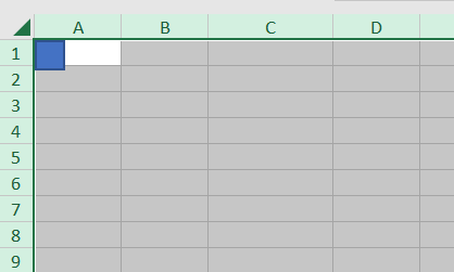
Step7: hover the mouse over the right border of the Column A’s header cell. And when the cursor turns into a double-arrow, drag the border until same to the rectangle. And then adjust Row1’s height same to the rectangle.

Step8: you should see that excel will adjust all the selected rows and columns.

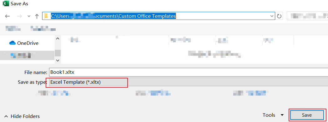
Step9: click on the File tab, and click Save As menu to save this workbook to your local disk as a template, you need to select Excel Template from the drop down list in the Save As dialog box.