VLOOKUP function is very strong and we often use this function in our daily life. And we all know that we can use VLOOKUP to get proper value by entering a value which is exactly the same with the lookup value in selected lookup range. If the entered value is not exactly matching the lookup value, we may get an error as returned value. So, we need to know how can we use lookup value by entering a partial match value in VLOOKUP. Don’t worry, this article will help you solve this problem.

First, let’s see an example.

Table 1:                                                                                 Table 2:

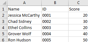
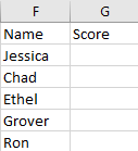
In above table 1, A column lists all students’ full names. But in table 2, F column only lists students’ names instead of the full names. So, if we enter

=VLOOKUP(F2,$A$2:$C$6,3,FALSE)

to lookup corresponding score for each student, we may get #N/A here.

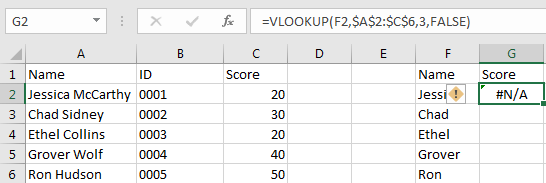
You may see we can set VLOOKUP parameter ‘Approximate Match’ here. Let’s see the result.

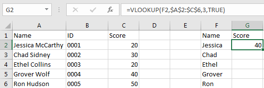
Unfortunately, we get an improper score this time.

VLOOKUP Partial Match in Excel

We still use above table to do demonstration here.

Step 1: In G2, enter the formula

 =VLOOKUP(F2&"*",$A$2:$C$6,3,FALSE).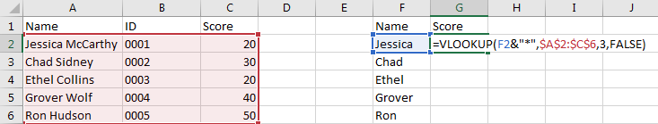

Step 2: Click Enter and let’s see the returned value.

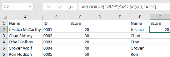
Now the returned score is correct.

Summary:

1. You can see in VLOOKUP parameter lookup_value, we entered F2&”*”, and use Exact Match to lookup information from lookup value. That means we can use partial match string with wildcard as lookup value.
2. The wildcard position depends on the missing part position of lookup value. There are three string and wildcards combinations, the format is like F2&”*”, “*”&F2, “*”&F2&”*”. Please see below examples for more details.

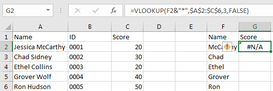
Example 1:

We change F2 name from Jessica to McCarthy and use the same formula to lookup score, this time we get #N/A. That’s because in the formula, lookup value is F2&”*”, string in F2 is listed in the front, “*” which stands for the other strings are listed at the last position, but actually McCarthy is not the first string in A1, so we get an error here.

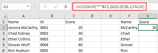
To solve this issue, adjust the position of string and wildcard, in this case, enter the formula

=VLOOKUP("*"&F2,$A$2:$C$6,3,FALSE)

then we can get correct score for F2.

Example 2:

If the string is listed in the middle, we can set “*” at both sides of the string. See updated table below.

In above table F2, McCarthy is listed in the middle of all strings, so we need to change formula to

 =VLOOKUP("*"&F2&"*",A2:C6,3,FALSE)

Make sure F2 is listed in the middle, “*” lists on both sides.

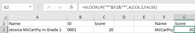
Now we can get correct score.

Video: Lookup Value by VLOOKUP Partial Match

This Excel video tutorial on performing partial matches with the VLOOKUP function in Excel. We’ll show you how to retrieve data even when you only have a part of the lookup value.

Related Functions

• Excel VLOOKUP function
  The Excel VLOOKUP function lookup a value in the first column of the table and return the value in the same row based on index_num position.The syntax of the VLOOKUP function is as below:= VLOOKUP (lookup_value, table_array, column_index_num,[range_lookup])….