How to Highlight Cell Which Its Adjacent Cell Value Equals to or Greater/Less Than It in Excel

In a two persons competition, we will record the scores for both sides, and then compare them to get the greater one, so we can confirm who is the winner. Actually, we can record two scores in two lists in excel, compare the two scores and highlight the greater one or the smaller one via excel ‘Conditional Formatting’ function. We can also highlight both cells if they have the same values. Based on this instance, this free tutorial will introduce you the way to highlight cell based on its adjacent cell value (highlight cell if its adjacent cell value is greater than or less than it, or even equals to it) in details step by step.

Precondition:

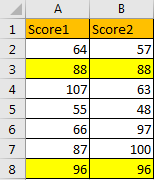
Prepare a table records two score lists.

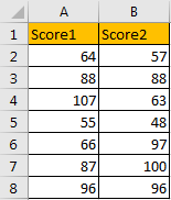
Part 1: Highlight Cells if Score1 Equals to Score2

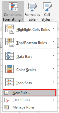
Step 1: Select the two score lists. Click Home in ribbon, then click Conditional Formatting in Styles group, select New Rule in menu.

Step 2: On New Formatting Rule dialog, select the last rule type: Use a formula to determine which cells to format.

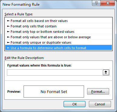
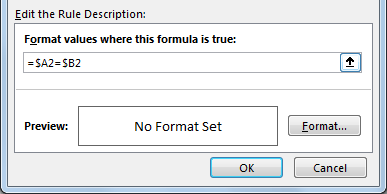
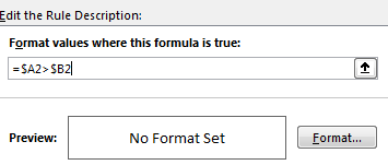
Step 3: In Edit the Rule Description section, in Format values where this formula is true textbox enter the formula =$A2=$B2.

Step 4: Click Format button in Preview section. Verify that Format Cells window is displayed.

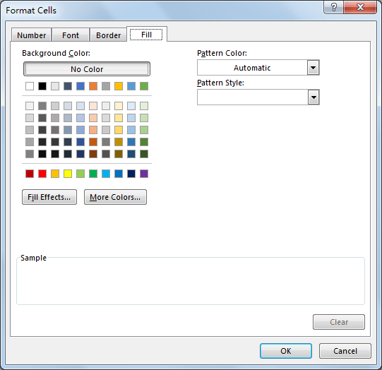
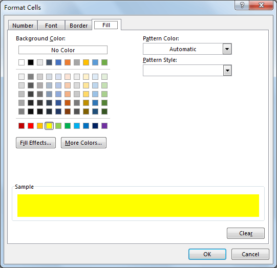
Step 5: Click Fill tab, then select a color as background color. For example, select yellow, then click OK.

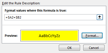
Step 6: After above step, we go back to New Formatting Rule window. You can see that in Preview section, cell is filled with yellow. Click OK.

Step 7: Verify that cells with the same scores are marked with yellow.

Part 2: Highlight Cells If It is Greater Than Its Adjacent Cells

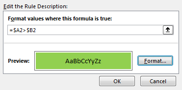
Step 1: Repeat above steps. Just a little different, in above step#3, enter the formula =$A2>$B2 in Format values where this formula is true textbox.

Step 2: Then select a color to mark cells, for example green.

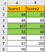
Step 3: Check the result. Verify that cells which score1 > score 2 are marked in green properly.

Part 3: Highlight Cells If It is Less Than Its Adjacent Cells

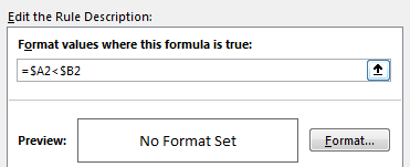
Step 1: Repeat above steps of ‘Part 1’. Just a little different, in above step#3, enter the formula =$A2<$B2 in Format values where this formula is true textbox.

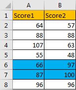
Step 2: Then select a color to mark cells, for example blue.

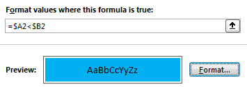
Step 3: Check the result. Verify that cells which score1 < score 2 are marked in blue properly.

You might also like:

How to Add Borders and Apply Format Automatically for Cells in Excel How to Apply Conditional Formatting across Workbook in Excel How to Create A Search Box to Show Matched Values in Excel How to Make Negative Numbers Red in Excel How to COUNT and SUM greater than and less than a number in Excel? How to Sum If Date is Greater or Less Than in Excel How to Find and Replace Values Greater Than or Less Than A Fixed Value in Excel How to Extract Data Which is Greater Than Value1 but Less Than Value2 in Excel How to Highlight All Error Cells in Excel How to Highlight All Non-Blank Cells in Excel How to Compare Two Columns and Highlight Duplicate Values in Excel How to Highlight Cells Based on Their First Letter/Character by Conditional Format in Excel