Sometimes when applying formula improperly, error like #N/A, #REF! will be displayed in cell, if we want to highlight all error cells how can we do? Though we can press ctrl and pick up all error cells one by one, this way is very bothersome. We need a convenient way. Actually, we can implement this via excel Conditional Formatting function, we can edit a new rule to filter all error cells and then highlight them. This article will show you the method in details.
Precondition:
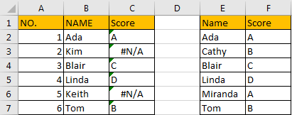
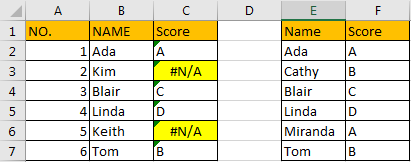
Prepare a table with some errors.
Method: Highlight All Non-Blank Cells by Conditional Formatting
Step 1: Select the table displayed in above screenshot.
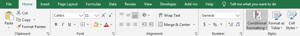
Step 2: Click Home in ribbon, click Conditional Formatting in Styles group.
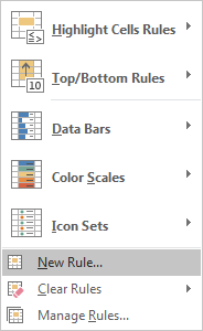
Step 3: Click the arrow on Conditional Formatting icon, select New Rule.
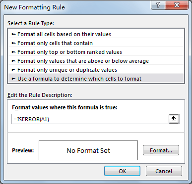
Step 4: In ‘New Formatting Rule’ dialog ‘Select a Rule Type’ pane, select ‘Use a formula to determine which cells to format’ option.
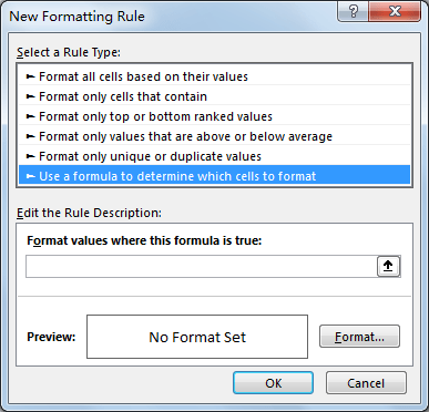
Step 5: Enter formula =ISERROR(A1) into ‘Format values where this formula is true.’.
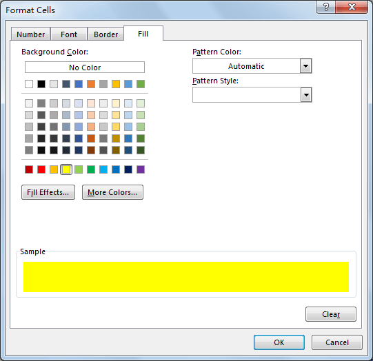
Step 6: Click Format button in Edit the Rule Description pane. On Format Cells, click Fill tab, select background color, then click OK to quit current dialog.
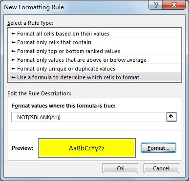
Step 7: In Preview field, you can see that cell is highlighted with yellow. Click OK to quit editing.
Verify that all error cells are highlighted properly.
Related Functions
- Excel ISERROR function
The Excel ISERROR function used to check for any error type that excel generates and it returns TRUE for any error type, and the ISERR function also can be checked for error values except #N/A error, it returns TRUE while the error is #N/A. The syntax of the ISERROR function is as below:= ISERROR (value)….