Sometimes in a column lists some numbers we need to filter values which are greater than one certain value and at the same time less than another value, and then extract them into another column. In this situation we can use Filter function to create number filter to filter data properly. In this article, we will show you the details to create number filter step by step.
Precondition:
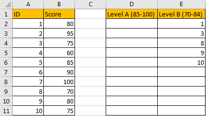
See table below. If we want to extract ID which score is in level B (greater than 69 and less than 85), we need to create number filter here.
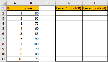
Table of Contents
1. Extract Data by Create Number Filter
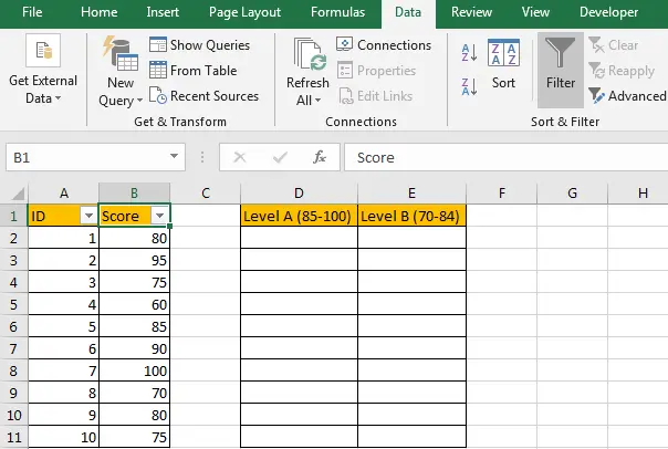
Step1: Create a filter on column B. Select B1, click Data in ribbon, click Filter.
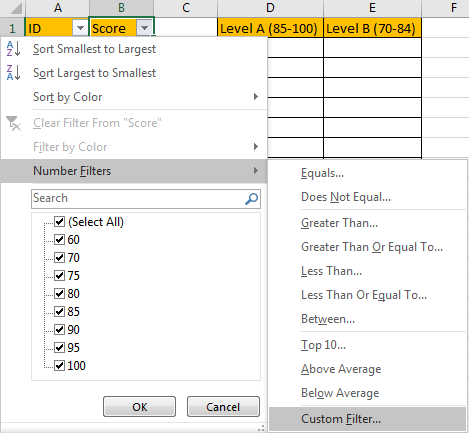
Step2: On B1 click Arrow button, then in filter menu click on Number Filters->Customer Filter.
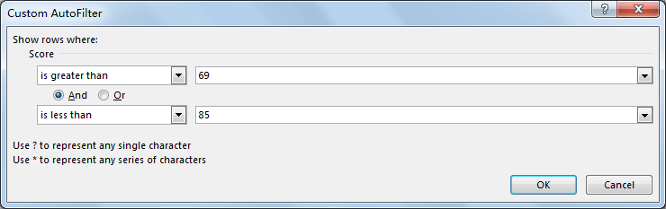
Step3: In Customer AutoFilter dialog, select ‘is greater than’ in dropdown list 1, then enter 69 as criteria in adjacent dropdown list; check on ‘And’, select ‘is less than’ in dropdown list 2, and then enter 85 as criteria in adjacent dropdown list.
Step4: Click OK. Verify that matched criteria values are filtered.
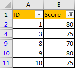
Step5: Press F5 to trigger Go To dialog.
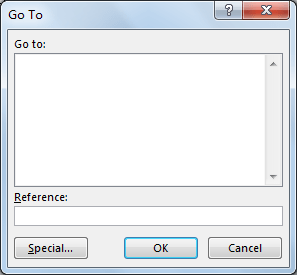
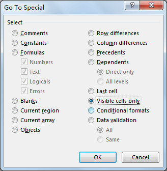
Step6: Click Special to load ‘Go To Special’ dialog, check on ‘Visible cells only’. Click OK.
Step7: On column A, select the visible range, press Ctrl+C to copy visible cells, then paste them in another worksheet.
Step8: Clear filter, all rows are expanded properly. Then copy values from another worksheet back to Level B column properly. Now all IDs match level B criteria are extracted.
2. Extract Data Using VBA Code
Now, let’s transition to the second method, where we’ll delve into the realm of VBA to craft a custom solution for extracting data within a specified range.
For a personalized and efficient approach, we’ll create a custom User Defined Function (UDF) using VBA.
Press ‘Alt + F11‘ to open the Visual Basic for Applications editor.
Click ‘Insert‘ and choose ‘Module‘ to create a new module.
Paste the following VBA code for the UDF:
Function ExtractIDsBetweenValues(rngIDs As Range, rngScores As Range, Value1 As Double, Value2 As Double) As Variant
    Dim resultArray As Variant
    Dim i As Long, j As Long
    Dim counter As Long

    ReDim resultArray(1 To Application.WorksheetFunction.CountIf(rngScores, ">" & Value1 & "") * Application.WorksheetFunction.CountIf(rngScores, "<" & Value2 & ""), 1 To 1)

    For i = 1 To rngScores.Rows.Count
        If rngScores.Cells(i, 1).Value > Value1 And rngScores.Cells(i, 1).Value < Value2 Then
            counter = counter + 1
            resultArray(counter, 1) = rngIDs.Cells(i, 1).Value
        End If
    Next i

    ExtractIDsBetweenValues = resultArray
End Function
This UDF, named ‘ExtractIDsBetweenValues,’ takes the ID range (rngIDs), the score range (rngScores), and the specified values (Value1 and Value2). It returns an array containing the extracted IDs meeting the score criteria.
Save and close the editor.
You can then use this function in a cell like this:
=ExtractIDsBetweenValues(A2:A11, B2:B11, 69, 85)Adjust the ranges and values as needed to suit your data and criteria.
3. Video: Extract Data
This Excel video tutorial where we’ll uncover two powerful methods for extracting data falling between two specific values. Our first approach involves utilizing the ‘Filter’ feature, while the second method employs the efficiency of VBA (Visual Basic for Applications).