This post will guide you how to create dynamic interactive chart in Excel. How do I create an interactive chart using option buttons in Excel.

• Create Dynamic Interactive Charts
• Video:Create Dynamic Interactive Charts

Create Dynamic Interactive Charts

---

Assuming that you have a list of data in range A1:D4, and you want to create a dynamic interactive chart based on your data. You need to control option buttons to show your charts based on product name. How to do it. You just do the following steps:

#1 copy your original data and paste below the original table.

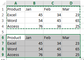
#2 delete all values from the newly table for each product.

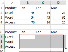
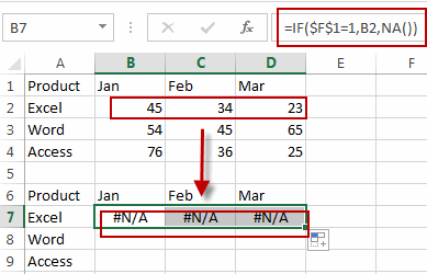
#3 Type the following formula in Cell B7 for product Excel. And drag the AutoFill Handle into the entire Excel row to apply this formula.

=IF($F$1=1,B2,NA())

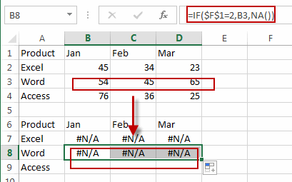
#4 Type the following formula in Cell B8 for product Word. And drag the AutoFill Handle into the entire Word row to apply this formula.

=IF($F$1=2,B3,NA())

#5 Type the following formula in Cell B9 for product Access. And drag the AutoFill Handle into the entire Access row to apply this formula.

=IF($F$1=3,B4,NA())

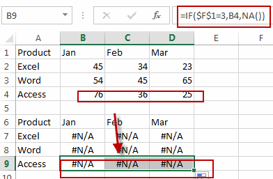
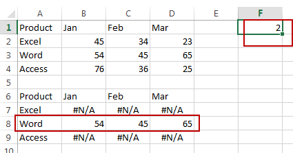
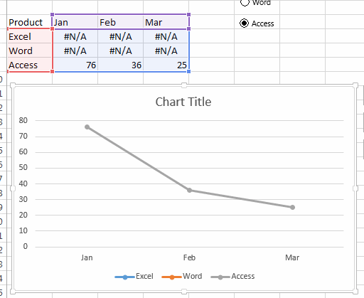
#6 Type number 1 or 2 or 3 in Cell F1, you would notice that your interactive data table is ready.  When you enter number 2 in F1, it will show your data for product word only.

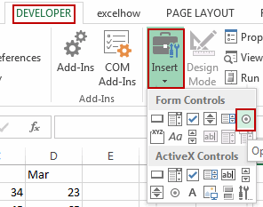
#7 go to DEVELOPER tab, click Insert command under Controls group. And click Option Button (Form Control) from the Form Controls section.

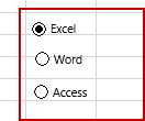
#8 and draw option buttons in your worksheet. And repeat this step to insert three option buttons and change the labels as Product names.

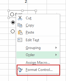
#9 right click on any of those radio buttons and select Format Control from the popup menu list. And the Format Control dialog will open.

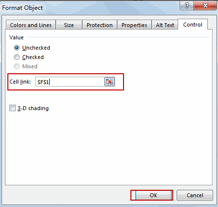
#10 click Control tab in the Format Control dialog, select Cell F1 in Cell link. And click Ok button.

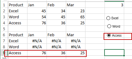
#11 then you can control your interactive data table using these option buttons.

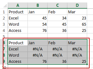
#12 select your interactive data table. And go to INSERT tab and insert a column or line chart.

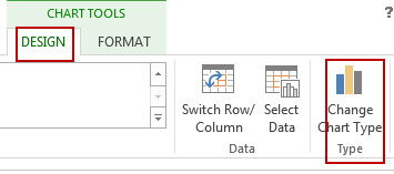
#13 select you chart, and go to Design tab, click Change Chart Type command under Type group. And the Change Chart Type dialog will open.

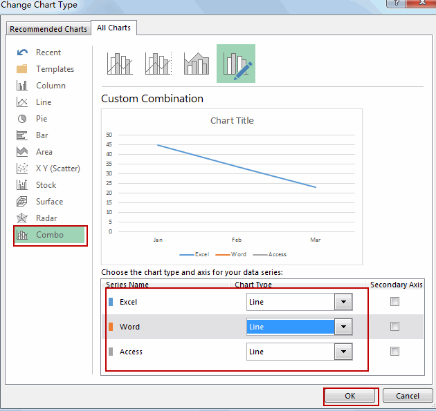
#14 select Combo menu in the Change Chart Type dialog, and choose the line chart or column chart type for all series.

When you click any of those buttons, it will show the relate chart.

Video:Create Dynamic Interactive Charts

 

Related Functions

---

• Excel IF function
  The Excel IF function perform a logical test to return one value if the condition is TRUE and return another value if the condition is FALSE.The syntax of the IF function is as below:= IF (condition, [true_value], [false_value])…