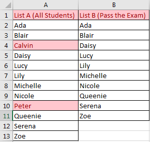
Suppose we have two lists, list A contains all students, list B only contains students who passed exam. So, list A is longer than list B, and students in list B are all included in list A. If we want to find out which student failed the exam, we can though compare the two list and find out the missing value to confirm the name list. Actually, in our work we often meet the situations that we need to compare two lists and find out the missing values. In this tutorial, we will help you to find out missing values via two ways, the first one is by Conditional Formatting function in excel, the second one is by using formula with VLOOKUP function.
Precondition:
Prepare two lists. List A contains all students. List B contains partial of them.
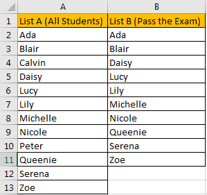
Table of Contents
Method 1: Compare Two Columns to Find Missing Value by Conditional Formatting
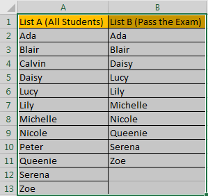
Step 1: Select List A and List B.
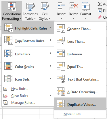
Step 2: Click Home in ribbon, click Conditional Formatting in Styles group.

Step 3: In Conditional Formatting dropdown list, select Highlight Cells Rules->Duplicate Values.
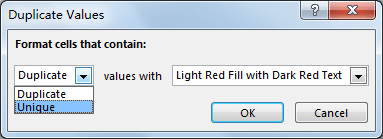
Step 4: In Duplicate Values dialog, select Unique in dropdown list. Keep default value in values with dropdown list. Then click OK.
Step 5: Verify that unique values are marked with dark red properly.
This way can be used in finding unique values from two lists.
Method 2: Compare Two Columns to Find Missing Value by Formula
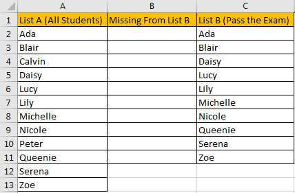
Insert a new column between List A and List B.
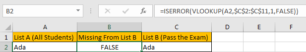
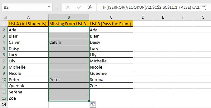
Step 1: In B2 enter the formula =ISERROR(VLOOKUP(A2,$C$2:$C$11,1,FALSE)). VLOOLIP function can help us to look up match value from List B. ISERROR function is used for checking whether match value exists or not, it returns TRUE or FALSE.
Step 2: Drag the fill handle down. Verify that B4 and B10 are filled with TRUE.
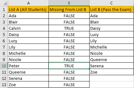
So, in List A, Calvin and Peter are students who failed in exam.
Step 3: If you want to show student name in new list directly, you can update formula =IF(ISERROR(VLOOKUP(A2,$C$2:$C$11,1,FALSE)),A2, “”).
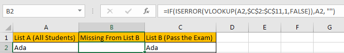
Step 4: After applying above formula for the following cells, missing value will display in new list directly.
Video: Compare Two Columns to Find Missing Value (Unique Value) in Excel
Related Functions
- Excel IF function
The Excel IF function perform a logical test to return one value if the condition is TRUE and return another value if the condition is FALSE. The IF function is a build-in function in Microsoft Excel and it is categorized as a Logical Function.The syntax of the IF function is as below:= IF (condition, [true_value], [false_value])…. - Excel VLOOKUP function
The Excel VLOOKUP function lookup a value in the first column of the table and return the value in the same row based on index_num position.The syntax of the VLOOKUP function is as below:= VLOOKUP (lookup_value, table_array, column_index_num,[range_lookup])…. - Excel ISERROR function
The Excel ISERROR function used to check for any error type that excel generates and it returns TRUE for any error type, and the ISERR function also can be checked for error values except #N/A error, it returns TRUE while the error is #N/A. The syntax of the ISERROR function is as below:= ISERROR (value)….