Suppose we have two lists, list A contains some products serial numbers, list B also contains some products serial numbers, and some of them are found in list A as well. So, there are some duplicate values in list A and list B. If we want to find them out, we can though compare the two list to find out the duplicate values. Actually, in our work we often meet the situations that we need to compare two lists and find out the duplicate values. In this tutorial, we will help you to fix this issue by two ways, the first one, we can use Conditional Formatting function in excel; the second one, we can use formulas.
Precondition:
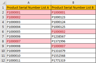
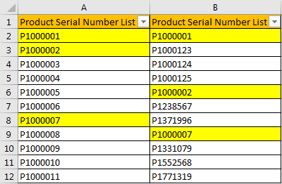
Prepare two columns. Column A and column B list product serial number. There are some duplicate values.
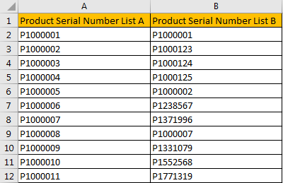
Table of Contents
Method 1: Compare Two Columns and Highlight Duplicate Values by Conditional Formatting Function
Step 1: Select List A and List B.
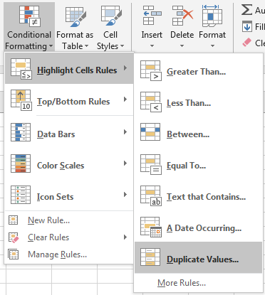
Step 2: Click Home in ribbon, click Conditional Formatting in Styles group.

Step 3: In Conditional Formatting dropdown list, select Highlight Cells Rules->Duplicate Values.
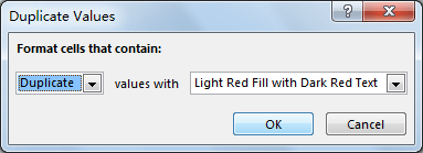
Step 4: In Duplicate Values dialog, select Duplicate in dropdown list. Keep default value in values with dropdown list. Then click OK.
Step 5: Verify that all duplicate values in both column A and column B are marked with dark red properly.
Method 2: Compare Two Columns and Highlight Duplicate Values by Formulas
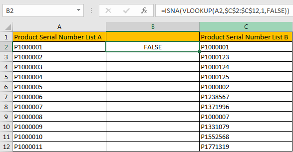
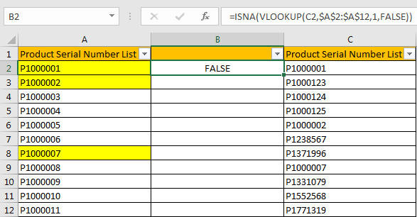
Step 1: Insert a new column between column A and column B. Then in B2, enter the formula =ISNA(VLOOKUP(A2,$C$2:$C$12,1,FALSE)). Click Enter, and we get FALSE.
In this formula, we can through VLOOKUP function to know whether value in column A exists in column B, if yes, VLOOKUP function will return matching value, otherwise it will return blank value, then we can use ISNA function (check whether a value is N/A) to get TRUE or FALSE value finally.
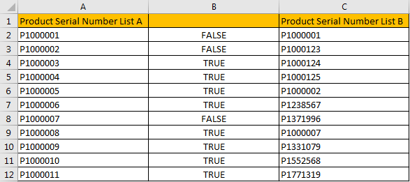
Step 2: Drag the fill handle down. Verify that B3:B12 are filled with TRUE or FALSE accordingly.
Step 3: Create a filter on column B. Click Data in ribbon, select Filter in Sort & Filter group.
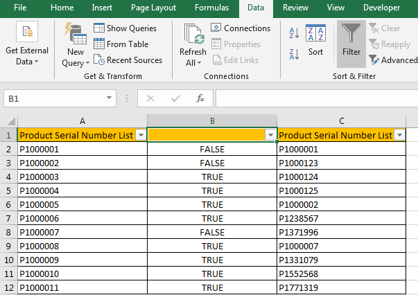
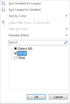
Step 4: Click filter arrow in B1. Only check on FALSE, click OK.
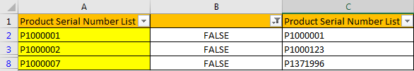
Step 5: After above settings, duplicate values are filtered. Fill them with yellow.
Step 6: Clear column B, then in B2 enter the formula =ISNA(VLOOKUP(C2,$A$2:$A$12,1,FALSE)).
Step 7: Repeat above steps#2-#5 to highlight duplicate values in column C.
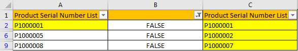
Step 8: Clear filter in column B. And delete column B. Verify that all duplicate values are highlighted.
Comment:
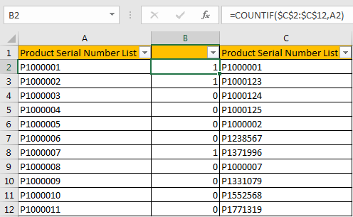
We can also use COUNTIF function here. Enter =COUNTIF($C$2:$C$12,A2) in B1, then we can get 1 for duplicate values or 0 for unique values.