In our daily life we often create tables for recording the money we spend for lunch or dinner or something else per date. This can help us know the total cost or average cost per date or other unit clearly via some statistic related functions in excel, and then we can cut back on unnecessary expenses and save our money.

Normally, one method for statistic in excel is creating pivot table. we can create a pivot table to auto calculate the total cost or average cost base on the values recorded in original table, and we can do filter by date or month or quarter to show different average cost for different period. Details see below screenshot.

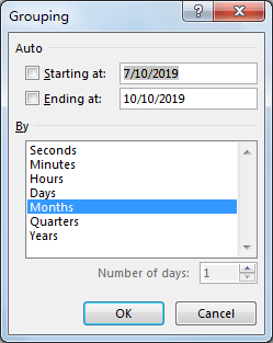
Obviously, Week is not listed in default grouping date list.

If you want to know the method for counting average data by week (without using pivot table), you can read below article, it can help you to solve your question.

1. Calculate Weekly Average by Formula in Excel

In Pre-Condition:

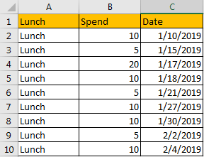
Prepare a simple table for demonstration. See screenshot below. You can see that we spend 10 or 5 or other values for lunch on different dates, some dates are included in one week. We want to count the weekly average for spend.

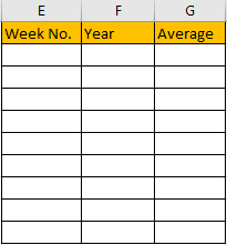
Step1: Create another table with three columns Week No., Year and Average. This table is used for recording the week number, year and the weekly average for launch spend.

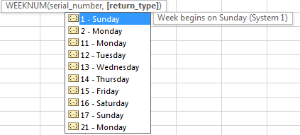
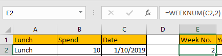
Step2: In E2, enter the formula =WEEKNUM(C2,2).

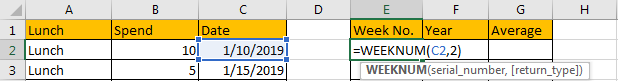
For function WEEKNUM, we set the second parameter as 2, that means week begins on Monday.

Step3: Click Enter to get returned value. We get 2 in this case. That means the date belongs to the second week in year 2019.

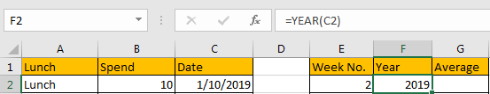
Step 4: In F2, enter the formula =Year(C2). We can get Year 2019.

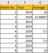
Step5: In G2, enter the formula:

=IF(AND(E2=E1,F2=F1),"",AVERAGEIFS($B$2:$B$10,$E$2:$E$10,E2,$F$2:$F$10,F2))

Then we get the returned value 10.

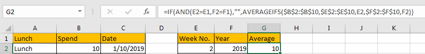
Comment: In this formula, we use AVERAGEIFS function to calculate the average by specific criteria, and use IF function to classify dates by week and then get according average. If (E2=E1,F2=F1) is true, then we get blank value, otherwise we will get the weekly average.

Step6: Drag the fill handle to fill the following cells in the table. We get weekly average values for all weeks.

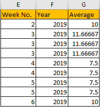
Comment: If you want to ignore Year, you can just enter the formula:

=AVERAGEIFS($B$2:$B$10,$E$2:$E$10,E2)

Then we can get below table. You can depend on your requirement to determine whether add or remove criteria.

2. Video: Calculate Weekly Average by Formula in Excel

In this video, we will learn how to calculate weekly averages based on dates and values within a week. Weekly averages represent trends and patterns in data.

3. Related Functions

• Excel WEEKNUM function
  The Excel WEEKNUM function returns the week number of a specific date, and the returned value is ranging from 1 to 53.The syntax of the WEEKNUM function is as below:=WEEKNUM (serial_number,[return_type])…
• Excel IF function
  The Excel IF function perform a logical test to return one value if the condition is TRUE and return another value if the condition is FALSE. The IF function is a build-in function in Microsoft Excel and it is categorized as a Logical Function.The syntax of the IF function is as below:= IF (condition, [true_value], [false_value])….
• Excel AND function
  The Excel AND function returns TRUE if all of arguments are TRUE, and it returns FALSE if any of arguments are FALSE.The syntax of the AND function is as below:= AND (condition1,[condition2],…)…