To calculate average with given criteria we can apply AVERAGIFS function. If the criteria or condition is a period for example one or more months, we can provide month information and then calculate average based on the given month. There are some date and time functions to return months or dates can represent a month. In this article, we will show you how to calculate average by month with AVERAGEIFS function, we use logical expressions with EOMONTH function to represent month.

In this article, we will introduce you the syntax, arguments and basic usage of above-mentioned functions, and use them to build a formula, and let you know the calculation steps of the formula.

1. EXAMPLE

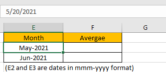
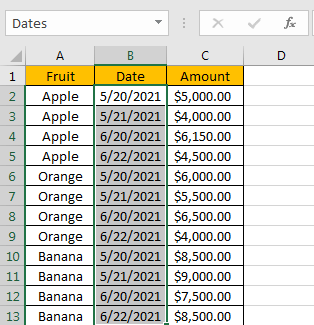
Refer to the left-hand side table, we can see some kinds of fruits are listed in “Fruit” column. Numbers in “Amount” column represent the sales on different dates. Dates belong to different months are recorded in “Date” column. In the right-hand side table, we want to calculate the average of amounts based on given months. In Month column, E2 and E3 are actually dates. For the following calculation we enter dates 05/20/2021 and 06/20/2021 into E2 and E3, and they are the earliest date shown in “Dates” column for May and June. But for looking clearly, we just show them in mmm-yyyy format and hide the date part.

To calculate the average of numbers based on given criteria, we need to apply AVERAGEIFS function here. In this case, our criteria is a whole month not a given period with start date and end date, so we can enter “DATE(2021,5,1)” as start date and “DATE(2021,5,31)” as end date. We can also apply EOMONTH function to return the last date of the given month.

Before creating a formula to calculate average value, we can name range references.

Select range B2:B13, in name box enter “Dates”, then press Enter.

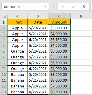
Select range C2:C13, in name box enter “Amounts”, then press Enter.

2. CREATE A FORMULA with AVERAGEIFS & EOMONTH FUNCTIONS

Step1: In F2, enter the below formula:

=AVERAGEIFS(Amounts,Dates,">="&E2,Dates,"<="&EOMONTH(E2,0))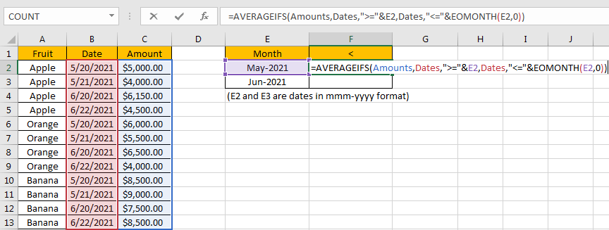

You can enter named range like “Amounts” into your formula directly, or you can also select the range by dragging the handle as well.

Step2: Press Enter after typing the formula.

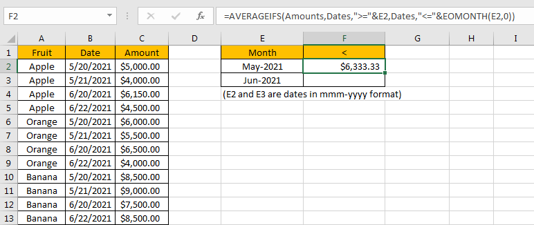
Pick up amounts from May, they are 5000 in C2, 4000 in C3, 6000 in C6, 5500 in C7, 8500 in C10, and 9000 in C11. Total 6 numbers. The average is (5000+4000+6000+5500+8500+9000)/6=6333.33. The formula works correctly.

3. FUNCTION INTRODUCTION

AVERGAEIFS function can be seen as AVERAGE+IFS. It returns the average of some numbers in range based on one or more given conditions or criteria.

Syntax:

=AVERAGEIFS (average_range, criteria_range1, criteria1, [criteria_range2], [criteria2], ...)

For AVERAGEIFS functions, it can handle wildcards like asterisk ‘*’ and question mark ‘?’; it also supports logical operations like ‘>=’,’<=’. If we need entering wildcards or logical operators to build criteria, they should be enclosed into double quotes (““).

EOMONTH function returns the last date for a given date.

Syntax:

 =EOMONTH(start_date, months)

Argument months is a serial number, n months represents n months before or after the start date. For example, if A1 is 05/20/2021, we enter =EOMONTH(A2, 1), it returns 06/30/2021 (set cell in proper date format). If we enter =EOMONTH(A2, -1) (negative value in months), it returns 04/30/2021. If we enter =EOMONTH(A2, 0), it returns 05/31/2021.

4. Formula EXPLANATION

AVERAGEIFS – average range

Named range “Amounts” is the average range in this case.

In the formula bar, select “Amounts”, press F9, values in this range are expanded in an array.

AVERAGEIFS – criteria range1/criteria range2

Named range “Dates” is the criteria range. We have only one criteria range in this case.

In the formula bar, select “Dates”, press F9, numbers which represent corresponding dates in this range are expanded in an array.

AVERAGEIFS – criteria range1

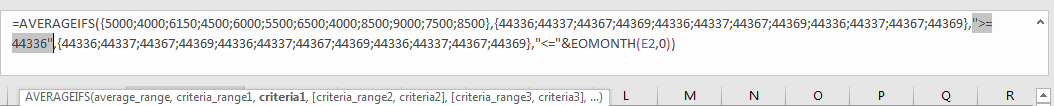
The first criteria is “>=”&E2. Date 5/20/2021 is recorded in E2, in logical expression “>=”&E2, E2 is converted to a five digits number which represents the date 5/20/2021. To concentrate operator “>=” and E2, we use “&” to connect them.

In the formula bar, select “>=”&E2, press F9, number 44336 is displayed instead of the date in E2.

AVERAGEIFS – criteria range2

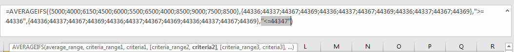
The second criteria is “<=”&EOMONTH(E2,0). EOMONTH function returns the last day of one month which is decided by the entered date. For E2 date is 5/20/2021, the second argument months is 0, so EOMONTH() returns the last day of May, it is 05/31/2021.

In the formula bar, select “<=”&EOMONTH(E2,0), press F9, number 44336 is displayed instead of the date 05/31/2021.

After explaining each argument in the formula, now we will show you how the formula works with these arguments.

After expanding values in each range reference, in the formula bar, the formula is displayed as:

=AVERAGEIFS({5000;4000;6150;4500;6000;5500;6500;4000;8500;9000;7500;8500},{44336;44337;44367;44369;44336;44337;44367;44369;44336;44337;44367;44369},">=44336",{44336;44337;44367;44369;44336;44337;44367;44369;44336;44337;44367;44369},"<=44347")

Now for the criteria range, we keep the numbers which can meet our two conditions “>=44336” and “<=44347”. So only numbers marked in bold meet our conditions.

{44336;44337;44367;44369;44336;44337;44367;44369;44336;44337;44367;44369}

For the qualified numbers, we mark “True” in the array, otherwise, “False” will be recorded. Then the original criteria range only contains “True” and “False”.

{True;True;False;Flase;True;True;False;Flase;True;True;False;Flase}

In logical expression, “True” is coerced to “1” and “False” is coerced to “0”. So, values in the array are converted to numbers:

{1;1;0;0;1;1;0;0;1;1;0;0}

After above steps, in current calculation step, we have two arrays.

{5000;4000;6150;4500;6000;5500;6500;4000;8500;9000;7500;8500}

– average range

{1;1;0;0;1;1;0;0;1;1;0;0}

– reference

Some numbers in average range are excluded in next calculation step if number’s corresponding value in reference range is 0. So only below numbers are kept and participate in next calculation step “calculate average”.

{5000;4000;0;0;6000;5500;0;0;8500;9000;0;0}

Calculate average of these number:

(5000+4000+6000+5500+8500+9000)/6=6333.33

5. Related Functions

• Excel AVERAGEIFS function
  The Excel AVERAGEAIFS function returns the average of all numbers in a range of cells that meet multiple criteria.The syntax of the AVERAGEIFS function is as below:= AVERAGEIFS (average_range, criteria_range1, criteria1, [criteria_range2, criteria2],…)….