VLOOKUP function is extremely strong among excel all functions. We often use it in our work for looking up match value. Sometimes when we autofill VLOOKUP we may get some errors. For most situations that’s because the selected range is entered incorrectly or changed automatically during filling process. This tutorial will help you to enter absolute reference or range name in VLOOKUP formula, then we can make sure autofill VLOOKUP function applies for all cells and works well, no error will be displayed.

1. Autofill VLOOKUP Correctly by Entering Absolute Reference in Formula

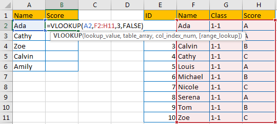
First, let’s see an example. In below table, we want to get match ‘Score’ from table E1:H11 for ‘Name’ in A column, and record the returned value in B column accordingly. So we can use VLOOKUP function here. After entering =VLOOKUP(), we can select A2 and range F2:H11 to fill the formula, then type 3 and FALSE to complete the formula.

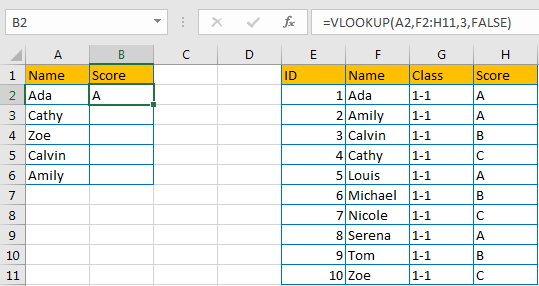
We can get the correct result A in B2 properly.

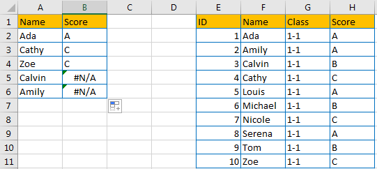
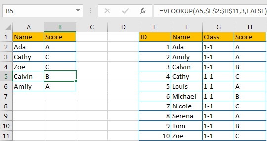
Drag the fill handle to B3:B6. Noticed that we get some errors.

Click B5 to check the formula. Noticed that reference (for table_array) is updated to F5:H14 automatically as relative reference is set up for cells by default. In this case, for Calvin, it is not included in its relative reference, so we get improper result here.

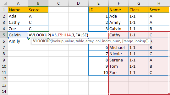
Above all, we need to keep table_array with a fixed value, so we need to update selected range as an absolute reference here, then autofill VLOOKUP will work properly.

Step1: In B2, enter the formula:

 =VLOOKUP(A2,$F$2:$H$11,3,FALSE)

After selecting range F2:H11, add $ manually before each character.

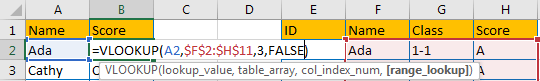
Step2: Drag fill handle down to fill other cells in B column. Verify that $ is copied with formula to other cells as well, and F2:H11 is not changed anymore in formula after adding $.

Comment:

In step 1, we can also press F4 after entering the formula, $ will be auto added in the formula.

2. Autofill VLOOKUP Correctly by Entering Range Name in Formula

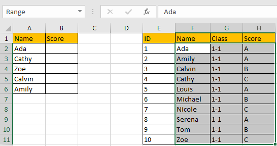
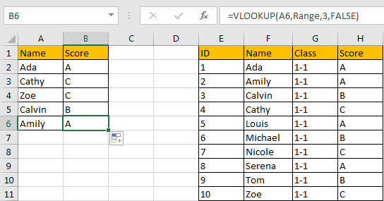
Step1: Select the range you want to apply VLOOKUP function, make sure the match value is listed in the first column in your selected range. In this example select F2:H11, then in Name Box (next to formula bar) type a name for this selected range, we name it ‘Range’ here.

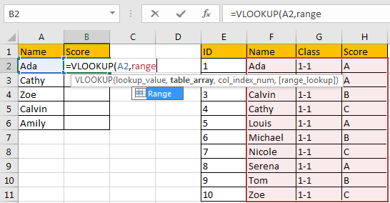
Step2: In B2, enter the formula:

 =VLOOKUP(A2,Range,3,FALSE)

You can see that when you entering ‘Range’ in formula, range table will be auto displayed properly.

Step3: Drag fill handle down to fill other cells in B column. All cells are filled with VLOOKUP properly and get correct values.

3. Video: Autofill VLOOKUP Correctly

This tutorial video will will show you why sometimes the auto fill doesn’t work correctly, and we’ll provide two methods to avoid the incorrect filling in Excel.

4. SAMPLE FIlES

Below are sample files in Microsoft Excel that you can download for reference if you wish.

5. Related Functions

• Excel VLOOKUP function
  The Excel VLOOKUP function lookup a value in the first column of the table and return the value in the same row based on index_num position.The syntax of the VLOOKUP function is as below:= VLOOKUP (lookup_value, table_array, column_index_num,[range_lookup])….