Sometimes we often create a table with different style or color of border to make table seems more standard or beautiful. Usually we often create a table with border before entering a value, normally in this case we already know the table range. Or we can add border for all cells with values after all values are entered into the selected range. If there is any way to add border automatically just after you finishing entering a value in the selected range? The answer is yes. And this article will show you the convenient way to add border automatically by Conditional Formatting function.

Suppose below table is what we want to show after value entry.

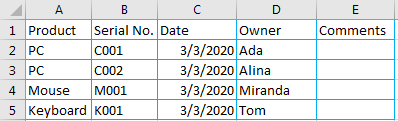
Cells are separated by light blue line gridline. So let’s try to add this type of border for each cell automatically now.

Add Borders Automatically by Conditional Formatting Function in Excel

---

Step 1: Select the range you want to create a table and apply the format for all cells. Refer to above table, we select the range A2:E5.

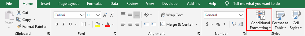
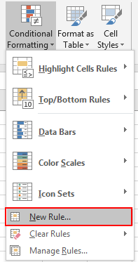
Step 2: Under Home tab, Styles frame, click Conditional Formatting ->New Rule.

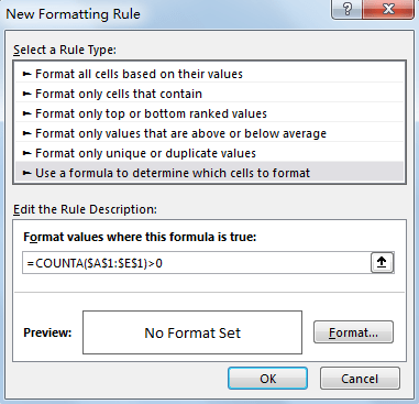
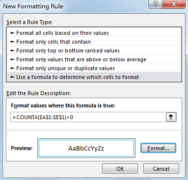
Step 3: In New Formatting Rule window, select the last Rule Type ‘Use a formula to determine which cells to format’. Obviously, we need to add a formula to define a rule in Rule Description text box, and if this formula is true, the format values will automatically be applied for the cells satisfy the rule.

Step 4: In ‘Format values where this formula is true:’ textbox, enter the formula =COUNTA($A$1:$E$1)>0. In the formula, $A$1:$E$1 is the first row in the range for cells apply the format. COUNTA function returns the number of non-blank cell. So if we enter a value into any cell in $A$1:$E$1, a table with defined format will be created.

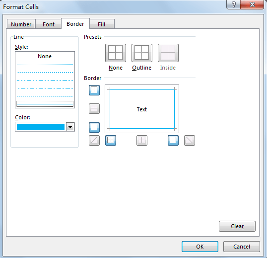
Step 4: Click Format button just next to Preview. Verify that Format Cells window is loaded. Click on Border tab, select line style and color in Line frame, then click Outline in Presets, verify that you can see the preview in Border frame. Cell is applied with light blue gridline.

Step 5: Click OK. Go back to New Formatting Rule window, verify that define format is displayed in Preview properly.

Step 6: Click OK and return to current worksheet.

Step 7: Select any cell in $A$1:$E$1, for example A1, enter a value ‘Product’.

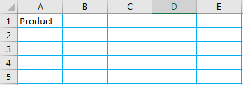
Verify that format is applied for all cells in selected range properly.

Note:

1. Step1 is the key point, you must to select the selected range before using Conditional Formatting function. Otherwise this function doesn’t work.
2. In Formula you can type any formula as long as it can meet your requirement.