This post will guide you how to use Google Sheets WORKDAY function with syntax and examples.
Description
The Google Sheets WORKDAY function returns a date or a serial number that represents a date that is the indicated number of working days before or after the starting date you specified. You can add a specified number of working days to the starting date and then returns a serial date. The working days will exclude weekends and any dates specified as holidays.
You can use the WORKDAY function to calculate working days and non-working days.
The WORKDAY function can be used to get a number representing the week of the year where the provided date falls in google sheets. The purpose of this function is to get the week number for a given date and it will return a number between 1 and 54.
The WORKDAY function is a build-in function in Google Sheets and it is categorized as a Date function.
Syntax
The syntax of the WORKDAY function is as below:
=WORKDAY(start_date, days, [holidays])
Where the WORKDAY function arguments are:
-
Start_date –This is a required argument. The starting date from which you want to count the number of working days. The date should be typed as a valid time a serial date.
-
days – This is a required argument. The number of working days that you want to add. A positive value for days yields a future date; a negative value yields a past date.
-
holidays – This is an optional argument. The list of holidays that you want to exclude from the working days. It can be a range of cells that contain the holiday dates or it can be a list of serial numbers that represent the holiday dates.
Note:
- If any argument is not a valid Excel date, a #VALUE! Error is returned.
- If start date value plus days is an invalid date, the WORKDAY function returns #NUM! Error.
- A serial date is how the google sheets stores dates and it represents the number of days since 1900-01-01, so the January 1, 1900 date is serial number 1 by default.
- If days value is not an integer number, it will be truncated.
Google Sheets WORKDAY Function Examples
The below examples will show you how to use google sheets WORKDAY Function to return the working days from the start date.
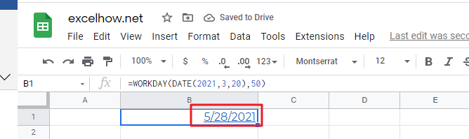
1# get the date 50 workdays from the starting date “3/20/2021”, enter the following formula in Cell B1.
=WORKDAY(DATE(2021,3,20),50)

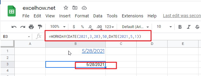
2# get the date 50 workdays from the starting date “3/20/2021”, excluding holidays 5/1/2021, type the following formula in Cell B2.
=WORKDAY(DATE(2021,3,20),50,DATE(2021,5,1))

Related Posts
Add Workdays in Google Sheets
To add or subtract workdays days from a date, respecting holidays but assuming a 7-day week: you can use the WORKDAY.INTL function with an argument that tells it how many days should be subtracted/added as well as which specific holidays ...
Google Sheets FLOOR Function
This post will guide you how to use Google Sheets FLOOR function with syntax and examples. Description The Google Sheets FLOOR function returns a number rounded down to the nearest multiple of significance. So it will return a rounded number. ...
Google Sheets EXP Function
This post will guide you how to use Google Sheets EXP function with syntax and examples. Description The Google Sheets EXP function returns e raised to the power of a number. The constant e is equal to 2.71828182845904, and it ...
Google Sheets FACT Function
This post will guide you how to use Google Sheets FACT function with syntax and examples. Description The Google Sheets FACT function returns the factorial of a given number. The factorial of a given number is equal to 1*2*3…* number. ...
Google Sheets EVEN Function
This post will guide you how to use Google Sheets EVEN function with syntax and examples. Description The Google Sheets EVEN function rounds a given number up to the nearest even integer. You can use the EVEN function to return ...
Google Sheets COUNTBLANK Function
This post will guide you how to use Google Sheets COUNTBLANK function with syntax and examples. Description The Google Sheets COUNTBLANK function use to count the number of empty cells in a range of cells. You can use the COUNTBLANK ...
Google Sheets DEGREES Function
This post will guide you how to use Google Sheets DEGREES function with syntax and examples. Description The Google Sheets DEGREES function converts radians into degrees. And it will return a numeric value. For examples, if you pass the PI() function into ...
Google Sheets COSH Function
This post will guide you how to use Google Sheets COSH function with syntax and examples. Description The Google Sheets COSH function returns the hyperbolic cosine of a given angle. The purpose of this function is used to get hyperbolic ...
Google Sheets COS Function
This post will guide you how to use Google Sheets COS function with syntax and examples. Description The Google Sheets COS function returns the cosine of a given angle. If you want to supply an angle to COS function in ...
Google Sheets COMBINA Function
This post will guide you how to use Google Sheets COMBINA function with syntax and examples. Description The Google Sheets COMBINA function returns the number of combinations for a given number of items and it includes repetitions. You can use ...