This post will guide you how to use Google Sheets ROW function with syntax and examples.

Description

---

The Google Sheets ROW function returns the row number of a cell reference.

The ROW function can be used return the row number of a specified cell in google sheets. The purpose of this function is to get the row number of a reference and It’s returned value is a number representing the row.

The ROW function is a build-in function in Google Sheets and it is categorized as a LOOKUP function.

Syntax

---

The syntax of the ROW function is as below:

= ROW ([reference])

Where the ROW function argument is:

• Reference – This is an Optional argument. the cell or range of cells reference that you want to get the row number.

Note:

• If the reference is omitted, the ROW function will return the row number of the current cell.
• Reference can be a single cell address or a range of cells.
• Reference can not include multiple cell references.
• If you want to get column number, you can use the COLUMN function.
• If you want to count rows, you can use the ROWS function.

Google Sheets ROW Function Examples

---

The below examples will show you how to use google sheets ROW Function to return the row number of a cell reference.
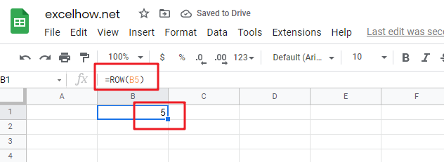
#1 To get the row number of “B5” cell in B1 Cell, just using the following ROW formula:

 =ROW(B5)

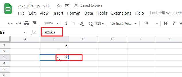
#2 To get the row number of the current cell, just using below formula:

=ROW()

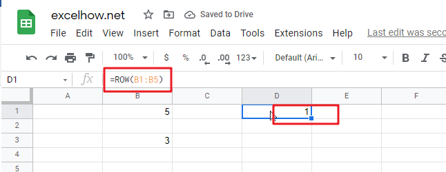
#3 get the first row number of range in excel

You can get the first row number in a range with an formula based on the ROW function as follows:

=ROW(Range)
=MIN(ROW(Range))

The ROW function will only display the first row number.