This article will introduce you how to use the RANK function in google sheets, and will show you a good example to better understand the usage of the RANK function.
Table of Contents
Google Sheets Rank Function Description
The Google Sheets Rank function is used to return the ranking of a given number from a list. If there are duplicate numbers in the list, then the numbers will be in the same rank.
The RANK function is a build-in function in Google Sheets and it is categorized as a Statistical Function.
Google Sheets Rank Function Syntax
The syntax of the Google Sheets Rank function is explained as follows:
= RANK (number,reference ,[order])
Where the arguments of the RANK function are as follows:
- Number – This is a required option, the number that you would like to get ranked
- reference – This is a mandatory option, it may be an array or cell region, or a cell reference contains the specified number
- Order – This is an optional, you can specify the number of 0 or 1 to determine the type of sorting; if the value of order is 1, it means that the RANK function will be sorted in ascending order, otherwise it will be ranked in descending order.
Google Sheets RANK Function Examples
The below examples will show you how to use Google Sheets RANK Function to get the rank of a given value within a supplied range of cells.
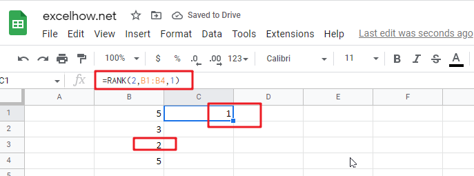
Example 1: If you want to get the sorting of number 2 in a given list B1:B4 in google sheets, then you can use the RANK function to do so with the following formula:
=RANK(2,B1:B4,1)

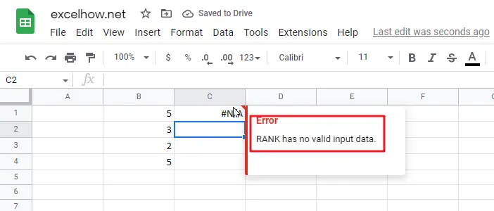
Note: The number 2 must be a value that exists in B1:B4, otherwise google sheets will report the error “Rank has no valid input data“.
