This post will guide you how to use Google Sheets HLOOKUP function with syntax and examples.
Table of Contents
Description
The Google Sheets HLOOKUP function lookup a value in the top row of the table and return the value in the same column based on index_num position. The lookup values must be in the first row of the table. HLOOKUP function supports approximate and exact matching.
The HLOOKUP function can be used to lookup across the first row of a table for a keyword and returns the value of a cell in the same column found in google sheets. The purpose of this function is to look up a value in a table, and the returned value is the matched value from a given table.
The HLOOKUP function is a build-in function in Google Sheets and it is categorized as a Lookup function.
Syntax
The syntax of the HLOOKUP function is as below:
= HLOOKUP (lookup_value, table_array, row_index_num,[range_lookup])
Where the HLOOKUP function arguments are:
- Lookup_value -This is a required argument. The value that you want to search for, in the first row of the table. Note: the lookup_value can be a value, a cell or ranges reference, or a text string.
- Table_array – This is a required argument. Two or more rows of data to be searched in the top row.
- Row_index_num – This is a required argument. The row number in table_array.
- Range_lookup – This is an optional argument. The value can be set as True or False. If true, the function will return an approximate match value. If False, it will find an exact match or it will return an error value #N/A.
Google Sheets HLOOKUP Function Examples
The below examples will show you how to use google sheets HLOOKUP Function to retrieve a value from a horizontal data table.
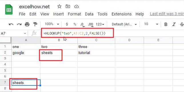
#1 To search “two” text string in row 1 and returns the value from row 2 that is in the same column, just using the following formula:
=HLOOKUP("two",A1:C2,2,FALSE())