This post will guide you how to use Google Sheets GETPIVOTDATA function with syntax and examples.
Table of Contents
Description
The Google Sheets GETPIVOTDATA function extracts specific data from a pivot table corresponds to the specified row and column name.
The GETPIVOTDATA function can be used to retrieve an aggregated value from a given pivot table by row or column name in google sheets. The purpose of this function is to extract data from a pivot table and the returned value is the data the you requested.
The GETPIVOTDATA function is a build-in function in Google Sheets and it is categorized as a Lookup function.
Syntax
The syntax of the GETPIVOTDATA function is as below:
=GETPIVOTDATA(value_name, any_pivot_table_cell, [original_column, …], [pivot_item, …])
Where the GETPIVOTDATA function arguments are:
- Value_name -This is a required argument. The name of the value in the pivot table
- Any_pivot_table_cell – This is a required argument. A reference to a cell in the desired pivot table.
- Original_column – This is an optional argument. The name of the column in the pivot table.
- Pivot_item – This is an optional argument. The name of the row or column shown in the pivot table corresponding to Original_column that you want to get.
Note:
- Value_name must be enclosed in quotation marks or a cell reference to any cell that containing the text.
Google Sheets GETPIVOTDATA Function Examples
The below examples will show you how to use google sheets GETPIVOTDATA Function to retrieve data from a pivot table.
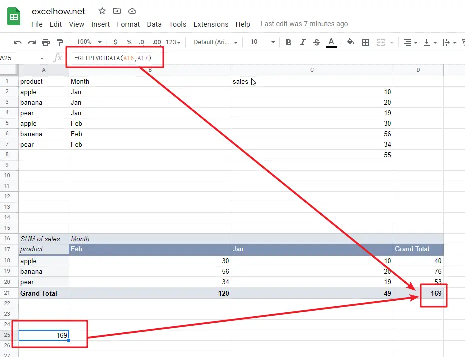
#1 Assuming that you have a pivot table in your google sheets, and you wish to get total sales from it, you can use the following GETPIVOTDATA function:
=GETPIVOTDATA(A16,A17)