This post will guide you how to use Google Sheets FIND function with syntax and examples.

Description

---

The Google Sheets FIND function returns the position of the first text string (sub string) within another text string.

The FIND function can be used when you want to get the position of a sub string inside another text string. It will return a number that indicates the starting position of sub string that you are searching in another text string. When searching text string is not found in another text string, the FIND function will return a #VALUE error in Google sheets.

The FIND function is a build-in function in Google Sheets and it is categorized as a Text Function.

Syntax

---

The syntax of the FIND function is as below:

= FIND(find_text, within_text,[start_num])

Where the FIND function arguments are:

• Find_text -This is a required argument. The text or substring that you want to find. (The string in the Find_text argument can not contain any wildcard characters)
• within_text -This is a required argument. The text string that is to be searched for the first occurrence of within_text
• start_num -This is an optional argument. It will specify the position in within text string where the search will start. If you omit start_num value, the search will start from the first character of the within_text string, in other words, it is set to be 1 by default. so you can use the google sheets Find function to look for the specified text starting from the specified position.

Notes:

• The Find function will return the position of the first character of find_text in within_text argument.
• If there are several occurrences of the find_text within another text string, it only returns the position of the first occurrence.
• If the find_text is an empty string, the position of the first character in the within_text is returned.
• If the find_text string is not found in within_text, it will return the #VALUE! Error.
• If start_number value is not greater than 0, it will return the #VALUE! Error value.
• The FIND function is case-sensitive. It means that uppercase and lowercase letters are different. For example, “find” will not match “FIND”. If you want to ignore case, use the SEARCH function in google sheets.
• The FIND function does not support wildcard characters, so if you want to use wildcard characters to find string, you can use SEARCH function in google sheets.
• You need to make sure that Find_text and within_text are not supplied in reverse order, or the #VALUE error will be returned.
• You can use the FIND function in combination with the IFERROR function to check for case when there are not matches within within_text.

Google Sheets Find Function Examples

---

The below example will show you how to use FIND function to find the position of a sub string within text string.

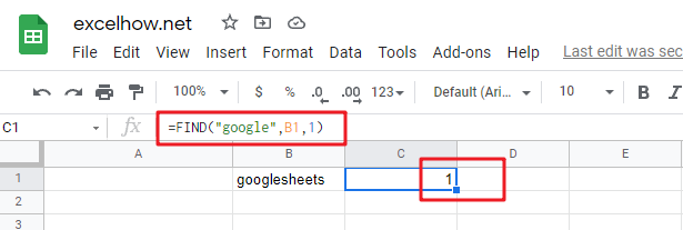
#1 To get the position of sub string “google” in cell B1, just using formula:

 =FIND("google",B1,1)

When you look for the text “google” in the Cell B1, it will return 1, which is the position of the first character of find_text “google” within the Cell B1.

#2 To get the position of sub string “google” in cell B1, starting with the ninth character, using formula:

=FIND("google",B1,9)

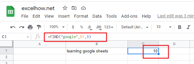
In the above example, it specified the start_num value as “9“, so you will get the position of the first character “g” of  the searched string “google”  within the value in Cell B1 when the starting position is 9. it returns 10.

#3 Finding “sheets” string in Cell B1, using the following Find formula:

=FIND("sheets",B1,1)

=FIND("sheets",B1,10)

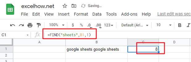
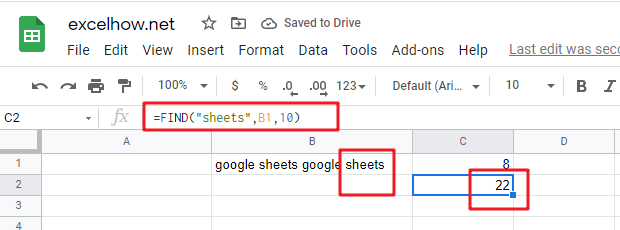
when you set the starting position as 1, it will return the position of the first “sheets” string in the value of Cell B1.

When you set the starting position as 10, it will return the position of the second “sheets” string in the value of Cell B1. The search will start from the tenth character of the value in Cell B1.

#4 Searching an empty string in Cell B1, using the following Find formula:

=FIND("",B1,1)

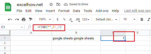
In the above example, when you look for an empty string in Cell B1 with the starting position as 1, and it will return the position of the first character of the within_text (the value of Cell B1).

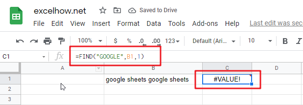
#5 Searching “find” text in Cell B1, using the following Find formula:

=FIND("find", B1,1)

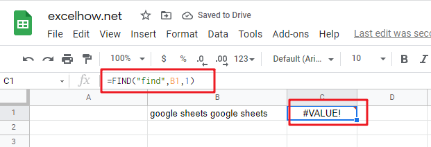
In the above example, when you look for the text “find” in Cell B1 and the string position is 1, it will return a #VALUE! error, As the searched string “find” is not found in Cell B1.

#6 Searching for a text as “google” in Cell B1 and the starting position is a negative number.

=FIND("google",B1,-1)

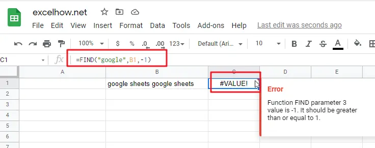
If the starting position is not greater than 0, it will return a #VALUE! Error.

#7 Searching for a string as “GOOGLE” in Cell B1, using the following formula:

=FIND("GOOGLE",B1,1)

As the FIND function in Google Sheets is case-sensitive, when you look for the string “GOOGLE” in Cell B1, the searched string “GOOGLE” is not found, the function will return a #VALUE! error.

Frequently Asked Questions

---

Question 1:  the FIND function returns a #VALUE error when it does not find the searched text within another string.  I want to know if there is another google sheets function in combination with the find function to handle the error message to return the actual value, such as: -1 or throwing others exceptions via returning values, like: -1,0 or FALSE.

Answer: As mentioned above, the FIND function is case-sensitive, and it can be combined with the ISNUMBER function and IF function to create a new IF  formula as follows:

=IF(ISNUMBER( FIND("google",B1)), FIND("google",B1), "not found")

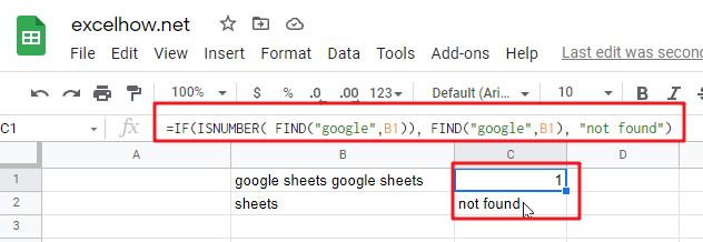
The FIND function will locate the position of the searched text “google” within Cell B1, and the ISNUMBER function will check the result returned by the FIND function if it is a number, if TRUE, then return TRUE, otherwise , returns FALSE. then the IF will check the Boolean value returned by ISNUMBER function, If TRUE, then returns the numeric position returned by the second FIND function, If FALSE, returns “not found” string.

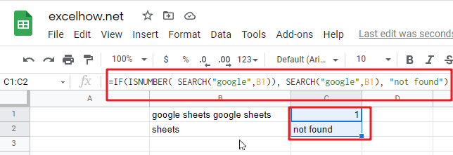
If you want a case-insensitive match and you can use the SEARCH function instead of the FIND function in the above formula:

=IF(ISNUMBER( SEARCH("google",B1)), SEARCH("google",B1), "not found")

Question 2: I want to extract a sub string from a string that separated by wildcard characters. I tried to use the below FIND formula to handle it. but it returned a #VALUE error message. Could you please help to check the below formula I used:

=RIGHT(B1,FIND("~**",B1))

Answer: you can use the following formula:

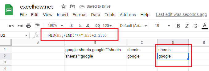
=TRIM(RIGHT(B1,Len(B1) - FIND("**",B1)-1))

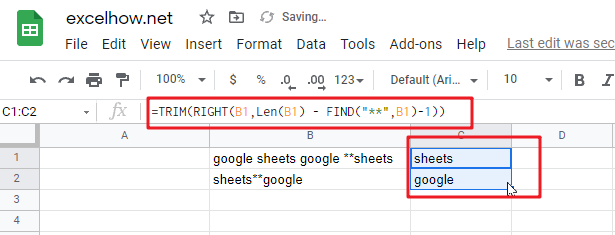
The find function will return the position of the first wildcard (**) character within a string in Cell B1. you need subtract the numeric position returned by FIND function from the length of the string in Cell B1 to get the length of sub string to the right of the wildcard character(asterisk). then the RIGHT function extracts the rightmost characters based on the length of sub string.

or you can use another formula to achieve the same result as follows:

=MID(B1,FIND("**",B1)+2,255)

Question 3: I am trying to extract the first word from another text string separated by space character. but it always return a #VALUE error message. I think it should be use the FIND function in combination with another function, such as: left function. but I still don’t know how to combine with those two functions to extract the first word.

Answer: right, you can create a google sheets formula that uses the FIND function and LEFT function. and you can use the below formula:

=IFERROR(LEFT(B1, FIND(" ",B1)-1),B1)

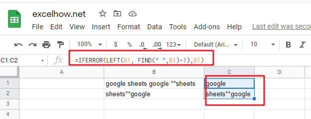
The find function returns the position of the first space character in the text string in Cell B1. the Formula “=FIND(” “,B1)-1 returns the numbers of the first word as the second arguments of the LEFT function.

If the text string in Cell B1 just only contains one word, then the find function will return #VALUE error. to handle this error, you need to use the IFERROR function, if the find function is not find the space character, then return the text string in B1. in other words, it just contains only one word in Cell B1.

Question 4: I am trying to extract an email address from a text string in Cell B1. how to write a google sheets formula to achieve the result.

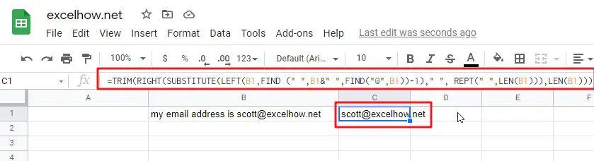
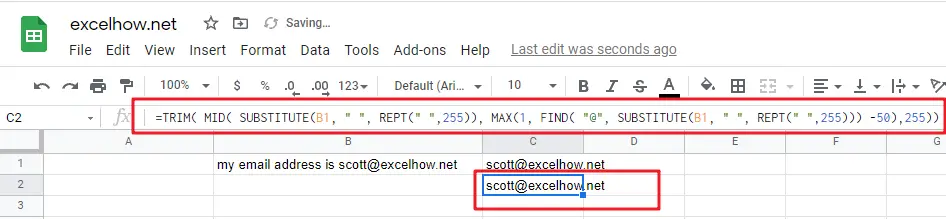
Answer: you can use a combination of the TRIM function, the LEFT function, the SUBSTITUTE function, the MID function, the MAX function and the REPT function to create a complex google sheets formula to extract email address from a string in Cell B1.

=TRIM(RIGHT(SUBSTITUTE(LEFT(B1,FIND (" ",B1&" ",FIND("@",B1))-1)," ", REPT(" ",LEN(B1))),LEN(B1)))

=TRIM( MID( SUBSTITUTE(B1, " ", REPT(" ",255)), MAX(1, FIND( "@", SUBSTITUTE(B1, " ", REPT(" ",255))) -50),255))

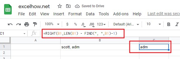
Question 5: I am trying to get the first name from a full name separated by a comma character. how to use a google sheets formula to extract the first name from a name as: “Last name, First name” format.

Answer: you can use a combination with the RIGHT function, the LEN function and the FIND function to create a google sheets formula to get the first name from a name. just using the following formula:

=RIGHT(B1,LEN(B1) - FIND(", ",B1)-1)