This post will guide you how to use Google Sheets CHOOSE function with syntax and examples.

Description

---

The Google Sheets CHOOSE function returns a value from a list of values based on index. For example, =CHOOSE(2,”google”,”sheets”,”book”) returns “sheets” value, and “sheets” value is the second value listed after the index number in this formula.

The CHOOSE function can be used to get a value from a list using a given index in google sheets. The purpose of this function is to get a value from a list based on a index and the returned value is the value at the given position.

The CHOOSE function is a build-in function in Google Sheets and it is categorized as a Lookup function.

Syntax

---

The syntax of the CHOOSE function is as below:

=CHOOSE (index_num, value1,[value2],…)

Where the CHOOSE function arguments are:

• index_num -This is a required argument. Specify the position number in the list of values.
• Value1,[value2] – This is a required argument.  A list of one or more values that you want to return

Note: 

• The index_num value must be a number between 1 and 29.
• If index_num value is less than 1 or greater than the length of the value list, the CHOOSE function will return #NUM!Error value.
• CHOOSE function will not retrieve values from a given range or array range
• Values can be an actual value or a cell reference.

Google Sheets CHOOSE Function Examples

---

The below examples will show you how to use google sheets CHOOSE Function to return a value from a value list based on a position value.

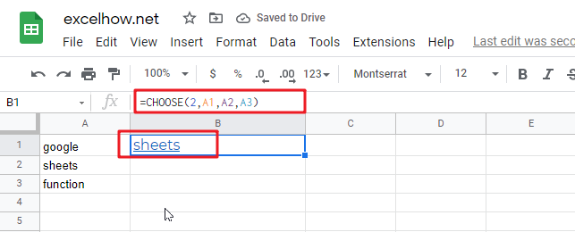
#1 To get the second value in the value list in B1 Cell, just using the following formula:

=CHOOSE(2,A1,A2,A3)

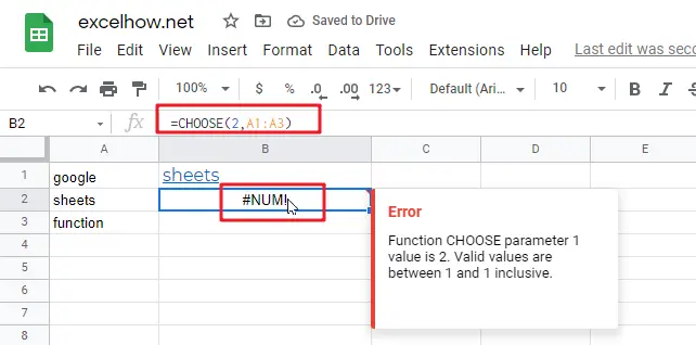
#2 CHOOSE function will not retrieve values from a cell range, and it will return a #NUM! Error, like the below formula:

=CHOOSE(2,A1:A3)

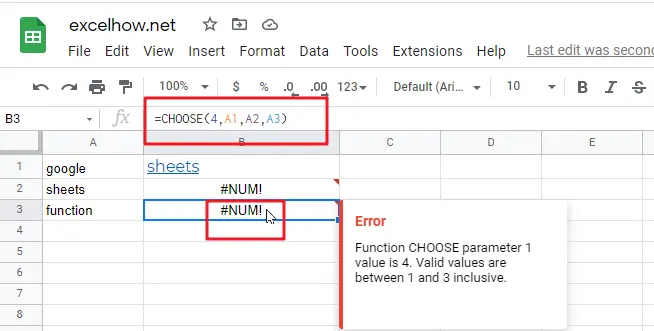
#3 INDEX number is out of range in CHOOSE formula, it will retrun a #NUM! error, like:

=CHOOSE(4,A1,A2,A3)