This post will guide you how to use Google Sheets CEILING function with syntax and examples.
Table of Contents
Description
The Google Sheets CEILING function returns a given number rounded up to the nearest multiple of a given number of significance. You can use the CEILING function to round up a number to the nearest multiple of a given number.
The CEILING function is a build-in function in Google Sheets and it is categorized as a MATH function.
Syntax
The syntax of the CEILING function is as below:
= CEILING (number, significance)
Where the CEILING function arguments are:
- number – This is a required argument. The number that you want to round up.
- significance – This is a required argument. The multiple of significance to which you want to round a number to.
Note:
- If either number and significance arguments are non-numeric, the CEILING function will return the #VALUE! Error.
- If the number argument is negative, and the significance argument is also negative, the number is rounded down, and it will be away from 0.
- If the number argument is negative and the significance is positive, the number is rounded up towards zero.
Google Sheets CEILING Function Examples
The below examples will show you how to use google sheets CEILING Function to round a number up to nearest multiple.
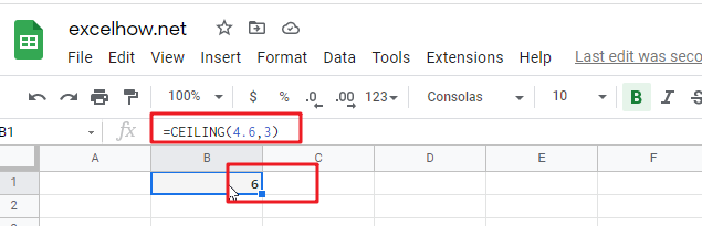
1# to round 4.6 up to nearest multiple of 3, enter the following formula in Cell B1.
=CEILING(4.6,3)
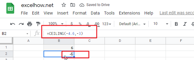
2# to round -4.6 up to nearest multiple of -3, enter the following formula in Cell B2.
=CEILING(-4.6,-3)
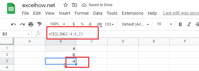
3# to round -4.6 up to nearest multiple of 2, enter the following formula in Cell B3.
=CEILING(-4.6,2)
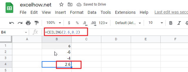
4# to round 2.6 up to nearest multiple of 0.2, enter the following formula in Cell B4.
=CEILING(2.6,0.2)
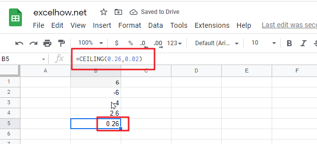
5# to round 0.26 up to nearest multiple of 0.02, enter the following formula in Cell B5.
=CEILING(0.26,0.02)