Suppose that you have a table consisting of a few cells with few values, and you want to filter out the set of records with the exact match concerning case sensitivity. You might take it easy and would prefer to manually filter out the desired case-sensitive match into another table without any need for the formula; then congratulations because you are thinking right.
But let me add that it would be a big deal while dealing with a bulk of data in the table, and then doing this bulky task manually would be a foolish decision.
But there isn’t any need to worry about it because after carefully reading this article, filtering out the set of records with the exact matches will be a piece of cake for you.
So let’s get straight into it!
Table of Contents
General Formula:
You can use the FILTER function in combination with the EXACT function to choose data records based on a case-sensitive match. The formula in F2 is written as follows:
=FILTER(total_data,EXACT(Filter_range,Filter_value))
Let’s See How This Formula Works:
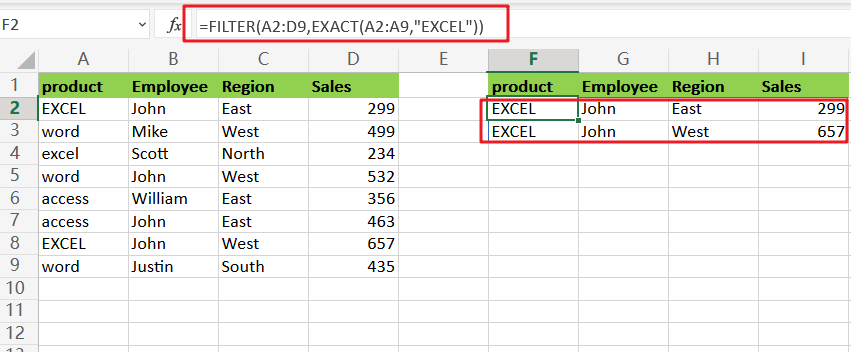
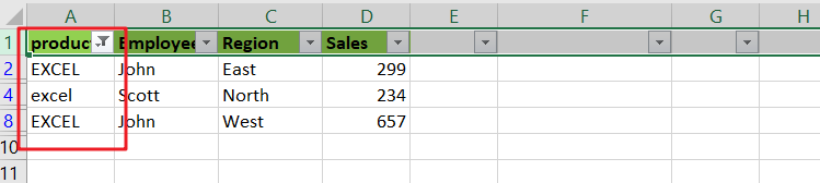
For example, suppose you got a task in which their table consists of Four columns (e.g., product, Employee, Region and Sales ) from which you need to filter out the data concerning the case sensitivity; Now let’s analyze how to write the formula and how this formula would do it.
As to extract the whole row of the product “EXCEL” respecting upper and lower case, so according to these requirements, we would write the formula as follows:
=FILTER(A2:D9,EXACT(A2:A9,"EXCEL"))
In the above formula, the FILTER function is used to get data based o the exact match. The array parameter is A2:D9, and it contains all of the data without the headers. The Include parameter is an EXACT function-based expression:
=EXACT(A2:A9,"EXCEL")
The EXACT function compares two case-sensitive text strings. If the two strings are identical, EXACT returns TRUE. If the two strings are not identical, EXACT returns FALSE, EXACT gives an array of 8 results, as seen below:
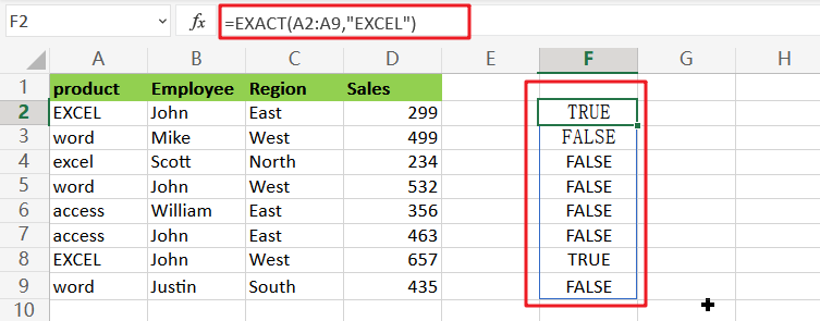
It’s worth noting that the location of TRUE values in this array correlates to the rows with the product “EXCEL”.
This array was returned straight to the FILTER function as the include parameter. FILTER filters the range A2:D9 using the array and returns the Four rows where the product is “EXCEL“. Rows with the product “excel” are excluded.
Following are the two other ways to Filter out data with an exact match in MS Excel:
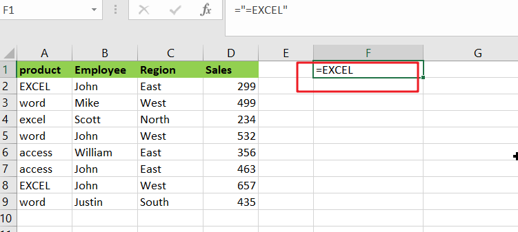
Using Excel’s Advanced Filter tool to Filter out data with an exact match
According to the given Example, we have the following range of data, and we want to do now is filter the cells whose content is “EXCEL”. Please do the following:
Step1: In the worksheet, create the criterion, and then to input the column header name that you want to filter, kindly use the Advanced Filter utility moreover this formula: =”=EXCEL” (EXCEL is the exact text you want to filter) underneath the herder cell, and click the Enter key, as seen in the screenshot:
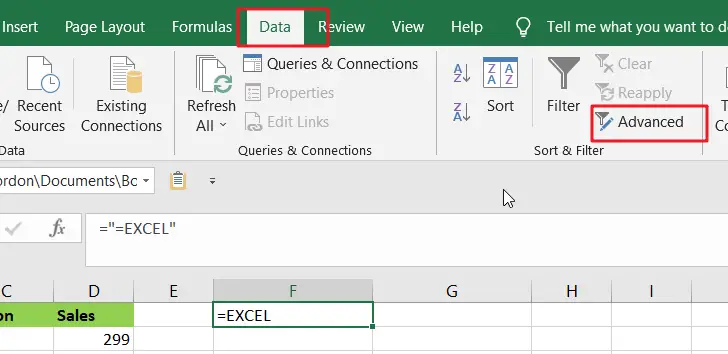
Step2: Then, as seen in the screenshot, go to Data > Advanced.
Step3: In the Advanced Filter dialogue box, choose Filter the list, in-place under the Action, and then specify the listed range to filter and the criterion range to filter based on, as shown in the screenshot:
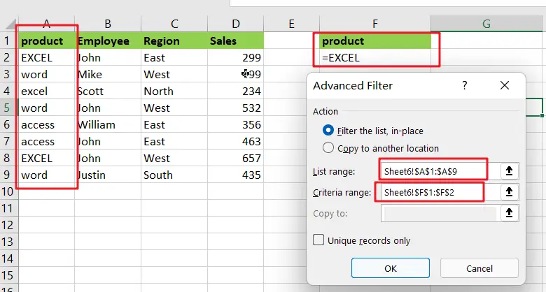
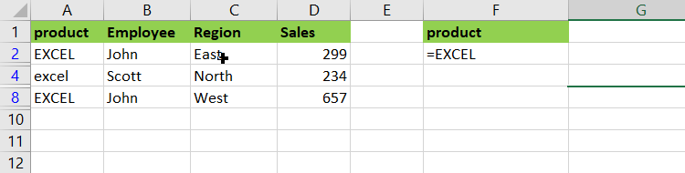
Step4: Then, after clicking the OK button, the precise text that you want will be filtered, as seen in the picture below:
Using the Custom Filter option to Filter out data with an exact match
In reality, the Auto Filter can also assist you in achieving the desired outcome.
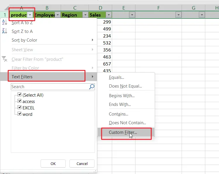
Step1: Choose the data range from which you wish to filter precise text.
Step2:To display the arrow button, go to Data > Filter.
Step3:Then, in the lower right corner of the cell, click the arrow button, and then pick Text Filters > Custom Filter, as seen in the screenshot:
Step4:In the Custom AutoFilter dialogue box that appears, choose equals from the drop-down list and input the text criteria that you wish to filter on, as shown in the screenshot:
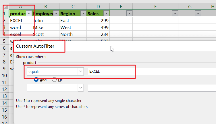
Step5:Finally, click the OK button to filter the exact text you want.
Related Functions
- Excel Filter function
The FILTER function extracts matched records from a collection of data using one or more logical checks. The include argument specifies logical tests, which might encompass a wide variety of formula conditions.==FILTER(array,include,[if empty])… - Excel EXACT function
The Excel EXACT function compares if two text strings are the same and returns TRUE if they are the same, Or, it will return FALSE.The syntax of the EXACT function is as below:= EXACT (text1,text2)…