Assume that in MS Excel, you have a table consisting of a few columns consisting of few values, and you want to filter to remove the specified columns from the table. You might take it easy and would prefer to manually filter out to remove the desired columns from the table, without any need for the formula; then congratulations because you are thinking right.
But let me add that it would be a big deal while dealing with multiple columns containing a bulk of data in the table, and then doing this bulky task manually would be a foolish decision.
But there isn’t any need to worry about it because after carefully reading this article, filtering out to remove the desired columns will be a piece of cake for you.
So let’s get straight into it!
Table of Contents
General Formula
To filter out desired columns from the table, we would use the FILTER function and supply the horizontal array; the general formula is as follows:
=FILTER(total_data,(range_name1=value1)+( range_name2=value2))
As we have altered the above formula according to the example which we would discuss in this article to understand that how this formula works and how to use this formula:
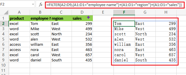
=FILTER(A2:D9,(A1:D1="employee name")+(A1:D1="region")+(A1:D1="sales"))
The end result is a filtered collection of data that only includes columns B, C, and D from the original data.
Let’s See How This Formula Works:
Although FILTER is usually used to filter rows, it may also filter columns; the secret is to give an array with the same number of columns as the original data. In this example, we use boolean logic, commonly known as Boolean algebra, to create the necessary array.
Multiplication corresponds to AND logic in Boolean algebra and addition corresponds to OR logic. In the following example, we use Boolean algebra using OR logic (addition) to target only the columns “employee name”, “region”, and “sales” as follows:
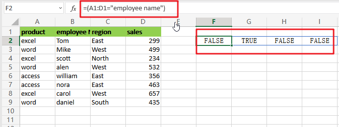
After evaluating each expression, we obtain three arrays of TRUE/FALSE values:
=(A1:D1="employee name")
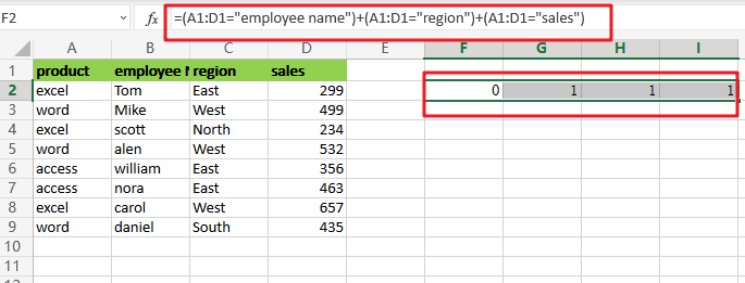
=(A1:D1="employee name")+(A1:D1="region")+(A1:D1="sales")
The arithmetic action (addition) turns TRUE and FALSE values to 1s and 0s, so think of it like this:
This is sent straight to the FILTER function as the include argument:
=FILTER(A2:D9,{0,1,1,1})
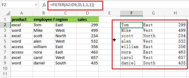
In the source data, there are 4 columns and 4 values in the array, all of which are either 1 or 0. FILTER utilizes this array as a filter to include columns 2, 3, and 4 from the given data. Column 1 has been eliminated. In other words, the only columns that remain are those linked with 1s.
Removing Columns Using the MATCH and Filter Functions
Applying OR logic with addition as demonstrated above works OK, but it does not scale well and makes it hard to utilize a range of numbers from a worksheet as the criterion. To create the include argument more quickly, you may use the MATCH function in conjunction with the ISNUMBER function as seen below:
=FILTER(A2:D9,ISNUMBER(MATCH(A1:D1,{"employee name","region","sales"},0)))

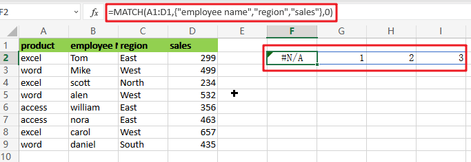
=MATCH(A1:D1,{"employee name","region","sales"},0)
The MATCH function is set to seek for all column headings in the array constants ,”employee name“,”region” and “sales” as illustrated. We implement it this way so that the MATCH result has dimensions consistent with the original data, which has 4 columns. Also, the third parameter in MATCH is set to 0 to force an exact match.
MATCH provides an array that looks like this when it runs:
=ISNUMBER(MATCH(A1:D1,{"employee name","region","sales"},0))
This array is sent straight to ISNUMBER, which produces another array:
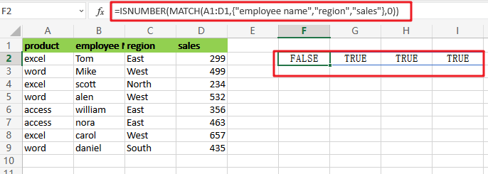
Like the one above, this array is horizontal and has 4 values separated by commas. Column 1 is removed using the array by FILTER.
Related Functions
- Excel ISNUMBER function
The Excel ISNUMBER function returns TRUE if the value in a cell is a numeric value, otherwise it will return FALSE.The syntax of the ISNUMBER function is as below:= ISNUMBER (value)… - Excel Filter function
The FILTER function extracts matched records from a collection of data using one or more logical checks. The include argument specifies logical tests, which might encompass a wide variety of formula conditions.==FILTER(array,include,[if empty])… - Excel MATCH function
The Excel MATCH function search a value in an array and returns the position of that item.The MATCH function is a build-in function in Microsoft Excel and it is categorized as a Lookup and Reference Function.The syntax of the MATCH function is as below:= MATCH (lookup_value, lookup_array, [match_type])….