If you are an valid MS Excel user, you have probably come across a situation where you wanted to filter the data in a separate table with specific criteria. You could do this task manually, which is also acceptable when dealing with a few data items. But if you got an assignment to filter out multiple items from a table consisting of a lot of data along with certain criteria, then doing these kinds of tasks manually would definitely be a stupid decision because this would not only waste your precious time, but you would also get tired of it and won’t complete your task on time.
But don’t be worry about it; for getting out of this fix and filtering out multiple data with specific criteria, all you have to do is read this article carefully.
So let’s dive into it.
Table of Contents
General formula:
The formula below would help you filter out multiple data with specific criteria within a few seconds.
As we have altered the following formula according to the example which we would discuss in this article to understand that how this formula works and how to use this formula:
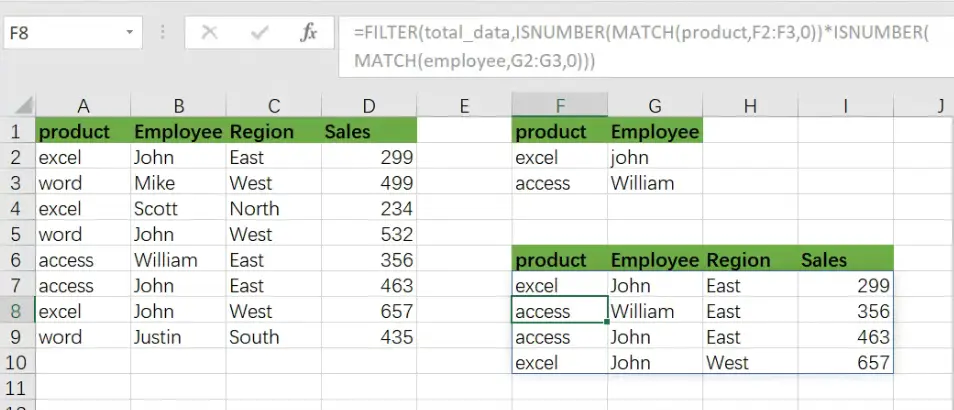
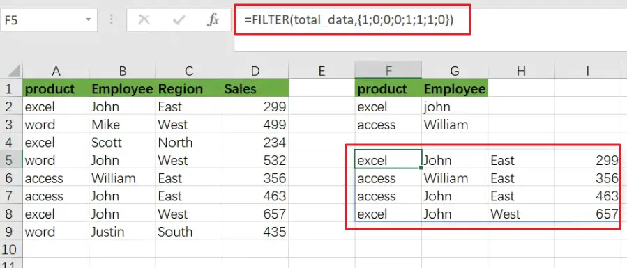
=FILTER(total_data,ISNUMBER(MATCH(product,F2:F3,0))*ISNUMBER(MATCH(employee,G2:G3,0)))
In the formula stated above, we are using the filter function along with the Match function, where ranges are specified for products(A2:A9), employee (B2:B9), and regions (C2:C9).
This formula produces information when the product is “excel” or “access”, AND the employee are “john” or “William”.
Syntax Explanation:
Before we dive into the formula for getting the job done effectively, we need to understand each syntax so that we can know how each syntax helps to Filter with multiple OR criteria :
Filter: This tool helps to narrow down or filter out a variety of data depending on user-defined criteria.Comma symbol(,): In Excel, this symbol functions as a separator and plays a vital role in separating a list of values.Parenthesis(): Its primary role is to group and separate elements.ISNUMBER: The ISNUMBER function determines if a value in a cell or a value derived from another formula is a number. ISNUMBER returns either “true” or “false.”MATCH: The MATCH function looks for a given item in a range of cells and returns the item’s relative location in the range.
Let’s See How This Formula Works:
Criteria for filtering out multiple data are entered in the range F2:G3 in this example. The formula’s rationale is as follows: the product is “excel” or “access”, AND the employee are “john” or “William”.
This formula’s filtering logic (the include parameter) is used with the ISNUMBER and MATCH functions and boolean logic in an array operation.
MATCH is set up “backward,” using lookup values from the data and criteria for the lookup array. For example, the first requirement is that the product be either “excel” or “access”. MATCH is configured as follows to apply this condition:
=MATCH(product,F2:F3,0) // look for excel product
As in the example, there are 8 values in the data; that’s why we get an array with 8 values that looks like the following:
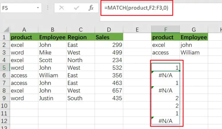
The above array would include #N/A errors (no match) or numbers (match). The numbers on the notice refer to either “excel” or “access” products. To turn this array into TRUE and FALSE values, the MATCH function is wrapped in the ISNUMBER function:
=ISNUMBER(MATCH(product,F2:F3,0))
which results in an array like the following one:
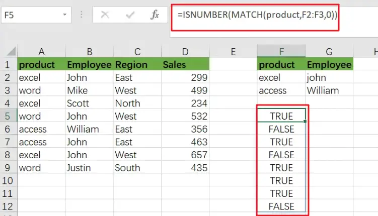
TRUE values in this array match a “excel” or “access”.
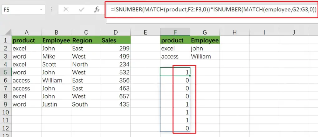
The exclusive formula has two expressions similar to the ones used for the FILTER function’s include argument.
Following the evaluation of MATCH and ISNUMBER, we get two arrays containing TRUE and FALSE values. The arithmetic action of multiplying these arrays together converts the TRUE and FALSE values to 1s and 0s.
Following the laws of boolean arithmetic, the outcome is a single array which is stated as follows:
which is sent as an argument to the FILTER function like the following:
=FILTER(B5:D16,{1;0;0;0;0;1;0;0;0;0;0;1})
Related Functions
- Excel ISNUMBER function
The Excel ISNUMBER function returns TRUE if the value in a cell is a numeric value, otherwise it will return FALSE.The syntax of the ISNUMBER function is as below:= ISNUMBER (value)… - Excel Filter function
The FILTER function extracts matched records from a collection of data using one or more logical checks. The include argument specifies logical tests, which might encompass a wide variety of formula conditions.==FILTER(array,include,[if empty])… - Excel MATCH function
The Excel MATCH function search a value in an array and returns the position of that item.The MATCH function is a build-in function in Microsoft Excel and it is categorized as a Lookup and Reference Function.The syntax of the MATCH function is as below:= MATCH (lookup_value, lookup_array, [match_type])….