In Excel, you can easily filter a table to display only the rows that meet your criteria. This is a quick way to find the information you need without scrolling through all the data. In this post, we’ll show you how to do it. Then, we’ll show you some other ways to filter data in Excel tables. Stay tuned!
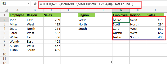
Table of Contents
General Formula:
=FILTER(total_data,ISNUMBER(MATCH(range1, filter_range,0)),"Not Found")Summary
When you want to include only records where the column equals one of many values, use a filter with ISNUMBER and MATCH functions. In this example shown G2 has:
=FILTER(A2:C9,ISNUMBER(MATCH(B2:B9, E2:E4,0))," Not Found ")Clarification:
The FILTER function has many different types of arguments, including numbers and matches. For example, The included argument can be created with an expression that uses ISNUMBER AND MATCH like this!
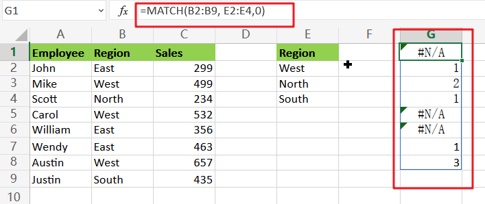
=MATCH(B2:B9, E2:E4,0)Try out this cool region finder for your request! MATCH can search inside the smaller range E2:E4, which means it will return an array like this:
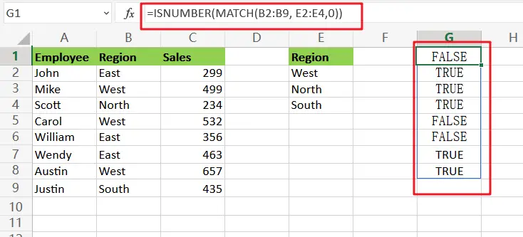
=ISNUMBER(MATCH(B2:B9, E2:E4,0))You can use this array to force a result of TRUE or FALSE by using the ISNUMBER function. The return value for this query is either 1 (true) if there are matching colors in positions corresponding with “found” numbers; 0(false).
When passing FILTER and including the argument that contains this filter, only rows with values corresponding to TRUE will be returned.
With Hardcoded Values:
The formula for this example is created with cell references, and it allows you to input colors in the E2:E4 range. However, an array constant can be used instead to produce the same result, Hardcoding values into your formulas!
=FILTER(A2:C9,ISNUMBER(MATCH(B2:B9, {"West","North","South"},0))," Not Found ")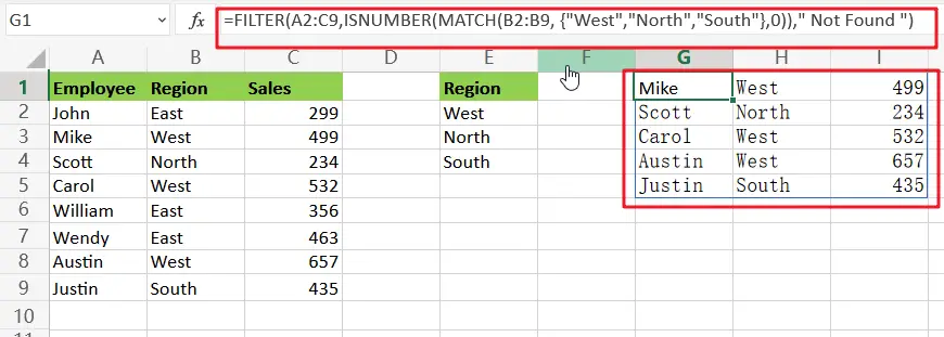
To Filter Multiple Values Use a Simple Filter:
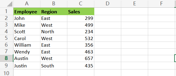
Using data from your company, this list shows which employee have been among region’s top sales.
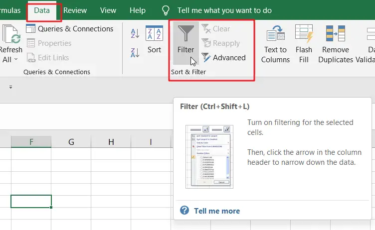
Clicking on any data point in our table will filter it, so clicking here could be useful for filtering out certain information or viewing only the newest records! First, go to the Data tab, select Sort & Filter and then Filter.
We can find a whole host of different items by clicking on these dropdown arrows, from which we’ll be able to make our selection.

Clicking on the filter in column one yields this image.
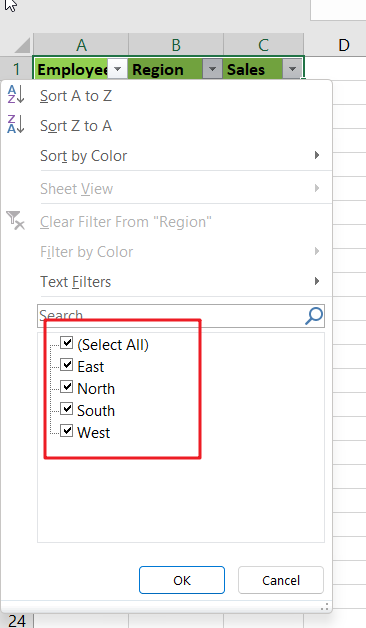
We need only click on West or East to select. This will deselect all other currently selected employee and allow us to choose between these two regsions.
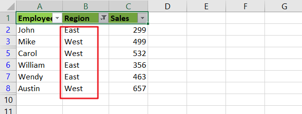
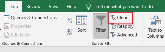
We’ll first clear the filter from our table by selecting any cell and clicking on the Filter tab again to filter out multiple values. You can notice that it is currently set to active with an icon background change:
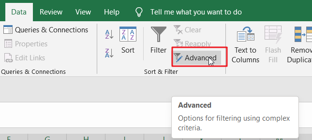
Advanced Filter To Filter Multiple Values
We will use Excel’s Advanced Filter to remove the filter from our table. We can find this option under Data >> Sort & Filter, right next to their regular filtering tools!
The window will appear when you click on it is quite interesting!
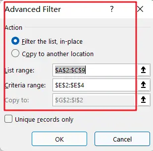
The Advanced Filter is a powerful tool to customize our results.
- We can choose between filtering in an existing table or copying filtered results into another location, called “copy.”
- We use the listed range in order to filter our table.
- We can use the criteria range field to define what we would like our filter’s result set to be.
- Copy to the designated location will write our filtered result.
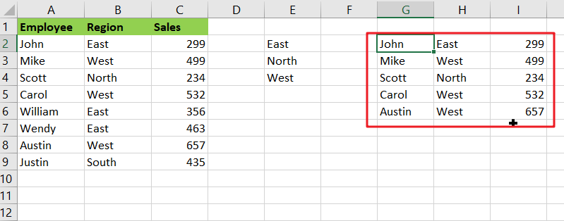
In this example, we will copy our filtered data set to cell G2. Our list range is A2:C9; criteria range E2:E4, and the copying happens in cells at positions where values meet or exceed those listed above them .
After you click OK, a new table will be created starting from the cell G2, and it’ll look like this:
Video: Filter Multiple Values
This Excel video tutorial where we’ll explore three distinct methods for filtering multiple values in your data – the dynamic ‘FILTER’ function, the classic ‘Filter’ feature, and the robust ‘Advanced Filter.’ Let’s dive into each method, starting with the formula-driven ‘FILTER’ function.
Related Function
- Excel MATCH function
The Excel MATCH function search a value in an array and returns the position of that item.The MATCH function is a build-in function in Microsoft Excel and it is categorized as a Lookup and Reference Function.The syntax of the MATCH function is as below:= MATCH (lookup_value, lookup_array, [match_type])…. - Excel Filter function
The FILTER function extracts matched records from a collection of data using one or more logical checks. The include argument specifies logical tests, which might encompass a wide variety of formula conditions.==FILTER(array,include,[if empty])… - Excel ISNUMBER function
The Excel ISNUMBER function returns TRUE if the value in a cell is a numeric value, otherwise it will return FALSE.The syntax of the ISNUMBER function is as below:= ISNUMBER (value)…