This post will guide you how to use the FILTER function to filter a value by column and then sort data by row in Microsoft Excel. You can use the following formula based on the SORT function in combination with the FILTER function to filter data by column and the sort data by row in Excel. the below is the general formula:
=SORT(FILTER(Range,(Table_Header_Range= oneHeader)+(Table_Header=oneHeader)),2,-1)
Or
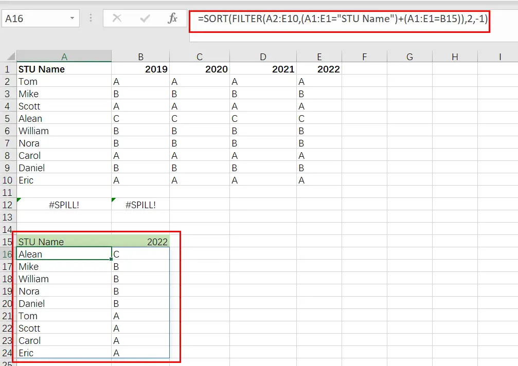
=SORT(FILTER(A2:E10,(A1:E1="STU Name")+(A1:E1=B15)),2,-1)
Let’s See How This Formula Works:
With this formula, you can sort and filter by column.
1) The heading (A1:E1="STU Name")+(A1:E1=B15) will keep the STU Name headings and add a year as a column heading, so there is a list of years for each STU Name.
2) -1 means to sort from smallest to largest. If you want to arrange value from largest to smallest, use 1 instead.
3) In the end, it will take all your data that has a value in that year and show it from smallest to largest. It will filter out all the others since they do not have a value inside them for that row/column combination, hence the term Filter By Column Formula!
In the below example, the formula in A16 is:
=SORT(FILTER(A2:E10,(A1:E1="STU Name")+(A1:E1=B15)),2,-1)
The above formula returns the STU Name column plus data for a year in B15, sorted by values.
Note: The FILTER function in Excel 365 is a new and improved way to restrict data. In earlier versions of the program, some alternatives could be used, but they were more complex than what you’ll find with this handy addition!
We’ll filter the data shown in A2:E10 by year and then sort it in this example. We also need to make sure that STU Name is included as well sorted in descending order like all of our other results! It is divided into two main steps:
- To filter, select the Matching Year and STU Name column
- Arrange the result of year values in descending order.
Filter By Column
To filter the data, we use a function called FILTER. This allows us to select only those rows where our conditions are met and remove any other non-matching values from that array so it will be smaller than what was originally inputted into Excel! To do this, just create an “include” argument that maps out how many columns should match to return identically-sized arrays with group names and year numbers replacing each other’s corresponding letter value (e). We can use a formula like the below one to return data for any year.
=FILTER(A2:E10,(A1:E1="STU Name")
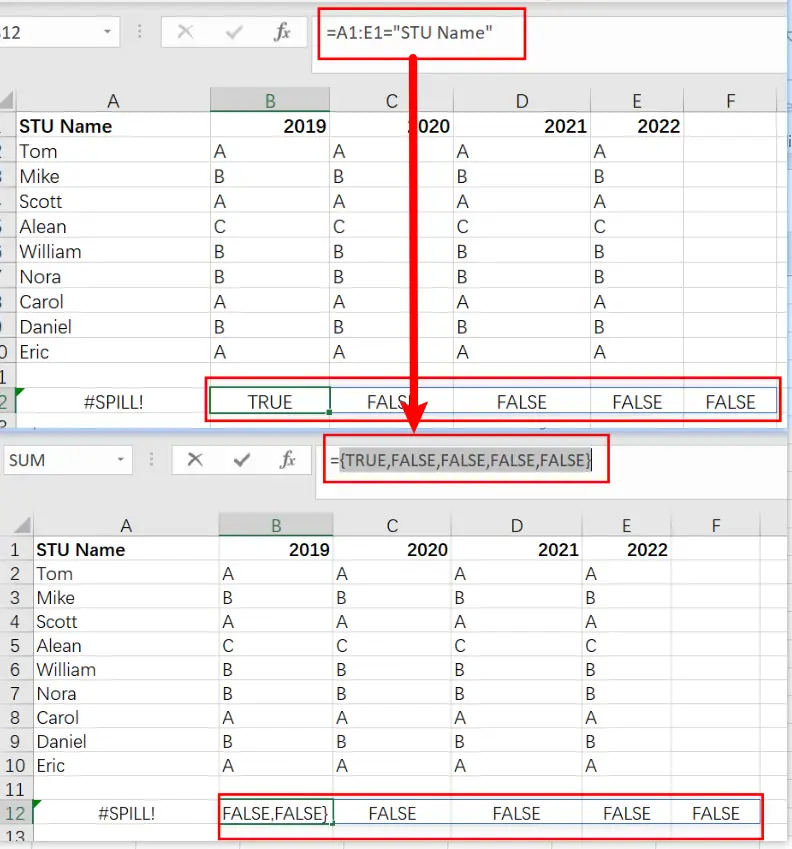
= A1:E1="STU Name" are the logical expression.
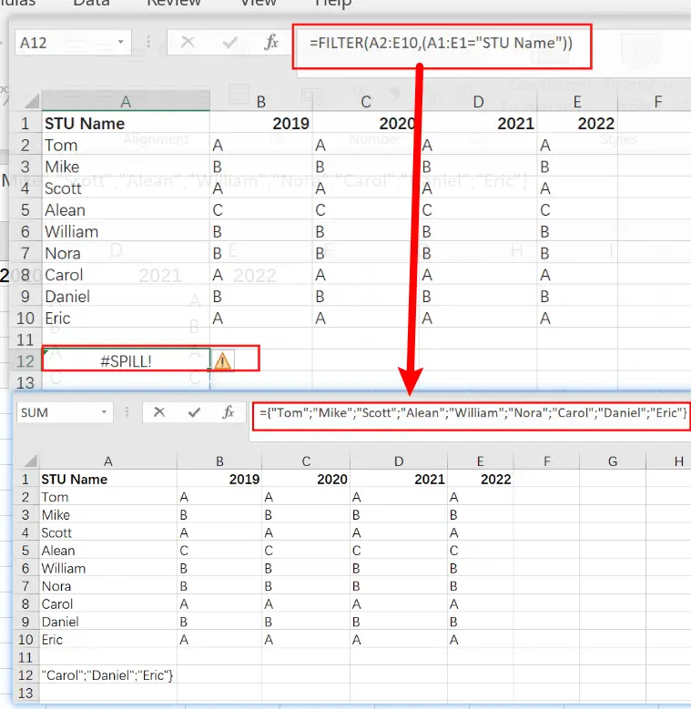
It returns an array with five columns.
{TRUE,FALSE,FALSE,FALSE, FALSE }
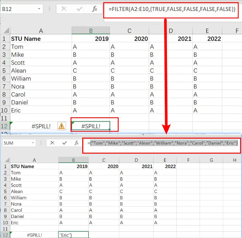
FILTER returns values for 2022 only when provided with the included argument.
FILTER(A2:E10,{ TRUE,FALSE,FALSE,FALSE, FALSE })
With the help of Boolean logic, we can work with TRUE and FALSE values like they were 1s or 0s. In Boolean algebra, addition corresponds to OR logic, and multiplication stands for AND. STU Name and year should both be returned when filtering on STU Name. This means we need OR logic – for example, a column equal to a ” STU Name ” OR equal to [year].
The result of using addition for OR logic is an expression like this:
=(A1:E1="STU Name")+(A1:E1=B15)
Joining two sets of TRUE and FALSE values with addition creates an array containing all the options.
The addition operation coerced the TRUE and FALSE into digits, creating a single array of 1s or 0’s:
{1,0,0,0,0,1}
When this array FILTER function applies as the include argument, it returns only two columns, 1 and 5 because only the first and five columns have 1 value while the second column is 0.
Sort by Row
The FILTER function, which is nested inside the SORT filter, returns two matching columns to be sorted.
=SORT(FILTER(A2:E10,(A1:E1="STU Name")+(A1:E1=B15)),2,-1)
In order to sort these columns by values in the year column (2022), we need an index number of 2 and a direction -1. When we use SORT, it sorts the data according to how much each value increases or decreases.
When the B15 year changes, the FILTER function ensures that new columns are selected and sorted.
Related Functions
- Excel Filter function
The FILTER function extracts matched records from a collection of data using one or more logical checks. The include argument specifies logical tests, which might encompass a wide variety of formula conditions.==FILTER(array,include,[if empty])… - Excel Sort function
The Excel SORT function in Excel sorts the contents of an array or range alphabetically or numerically by columns or rows.The syntax:=SORT(array, [sort index],) …