Suppose that you are in a situation where you need to filter out the top n values from the list having few values with specific criteria, or you can say that with a particular condition, and I am also pretty sure about it that you would definitely choose to do it manually, which is also a great choice when you have only a few values in a list, and you want to filter out the top n values with a certain criteria (condition).

But if you are dealing with multiple values in the list and you want to filter out the top n values with a specific criteria (condition), then in such a situation doing these tasks manually would be a foolish act because doing it manually, there are 90% chances that you would 100% get tired of it and can’t complete your task at the right time.

But don’t be worry about it because after carefully reading this article filtering out the top n values with the particular criteria (condition) from the list containing multiple values would become a piece of cake for you.

So let’s dive into the article to take you out of this fix.

General Formula

---

The Following formula would help you Filter on top n values with the specific criteria (condition) in MS Excel:

=FILTER(total_data,(condition_range>=LARGE(IF(condition),n))*( condition))

Syntax Explanations

---

Before going into the explanation of the formula for getting the work done efficiently, we must understand each syntax which would make it easy for us that how each syntax contributes to filtering out the top n values in MS Excel.

• Filter: This function contributes to narrowing down or filtering out a range of data on the user-defined criteria.
• total_data: In your worksheet, it represents the input ranges.
• Comma symbol (,): In Excel, this comma symbol acts as a separator that helps to separate a list of values.
• condition_range: In Excel, the range is nothing but the difference between highest and lowest values
• Parenthesis (): The core purpose of this Parenthesis symbol is to group the elements and separate them from the rest of the elements.
• Greater than Equal To Symbol (>=): Greater than Equal To Symbol (>=) is used to identify the values which are either greater than or equal to.
• LARGE: Large function is used to get the higher arguments.
• IF( ): IF function is the most popular function in excel, which checks whether the condition is met.
• Criteria: This means the condition to which the user desires to get the results according to it.

Let’s See How This Formula Works

---

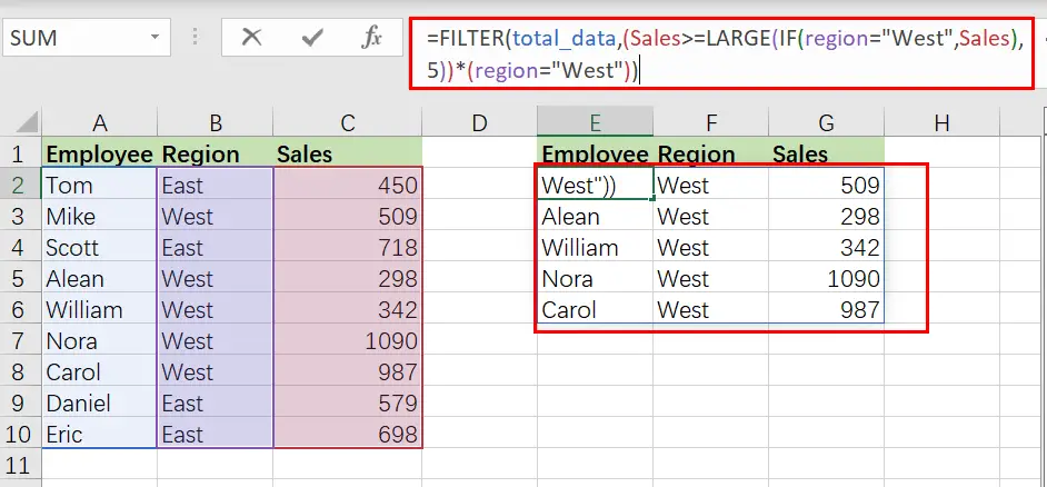
For instance, you got a task in which there is a table where you have candidates of some regions (i.e., region East and region West ) and which are assigned to a particular sales, now you want to filter out the top 5 candidates with the higher sales along with the criteria that those top 5 candidates must be from the region West, now let’s analyze that how to to write the formula and how this formula would do it.

As to filter on the top n values with criteria, we would write the formula according to the given list like:

=FILTER(total_data,( Sales >=LARGE(IF(region="West", Sales),5))*( region =" West"))

Here the region (B2:B10), Sales (C2:C10), and total_data (A2:C10) are the named ranges in the above example.

The FILTER function is used in this formula to obtain data based on a logical test built using the LARGE and IF functions. The top five sales in region West are the outcome.

The FILTER function uses the include parameter to apply criteria. Criteria in this example are built using boolean logic, as seen below:

=(Sales >=LARGE(IF(region="West", Sales),5))*( region =" West"))

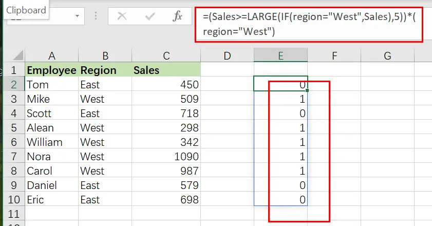
The expression’s left side seeks sales greater than or equal to the fifth-highest sale in region West:

=IF(region="West", Sales)

The IF function ensures that LARGE only works with region West sales. Because we have a total of 9 sales, IF produces an array with 9 outcomes, as seen below:

{FALSE;509;FALSE;298;342;1090;987;FALSE;FALSE}

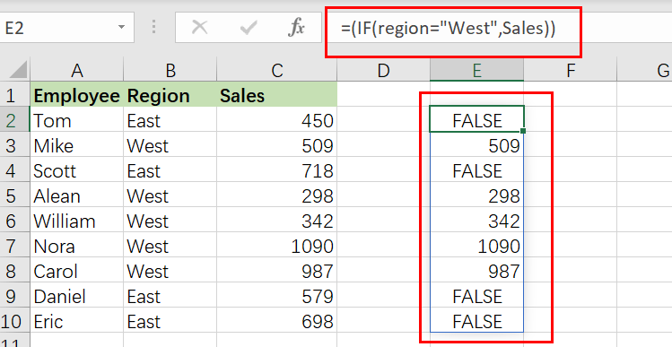
It’s worth noting that the only sales that survive the procedure are from region West. All other results are FALSE. As the array parameter, this array is returned straight to LARGE:

=LARGE({FALSE;509;FALSE;298;342;1090;987;FALSE;FALSE},5)

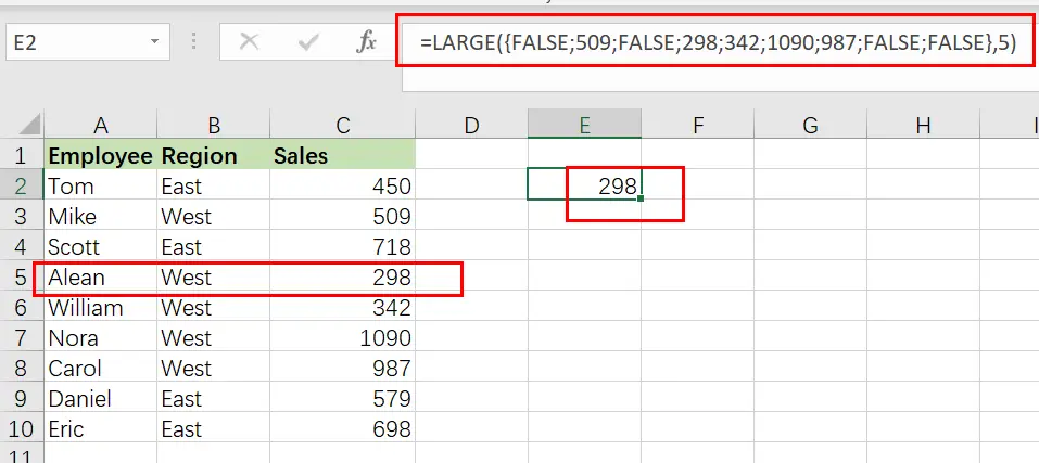
The FALSE values are ignored by LARGE, which yields the Fifth-highest sales, 298.

We can now reduce the formula to:

=FILTER(total_data ,(Sales>=298)*( region =" West"))

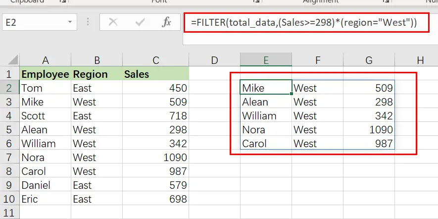
Finally, FILTER retrieves results in the E2:G6 range.

Sort results by Sales Value Using Sort Function

---

FILTER will return matched entries in the order they occur in the supplied data by default. To sort results by sales in decreasing order, nest the original FILTER formula within the SORT function as follows:

=SORT(FILTER(total_data,( Sales >=LARGE(IF(region="West", Sales),5))*( region =" West")),3,-1)

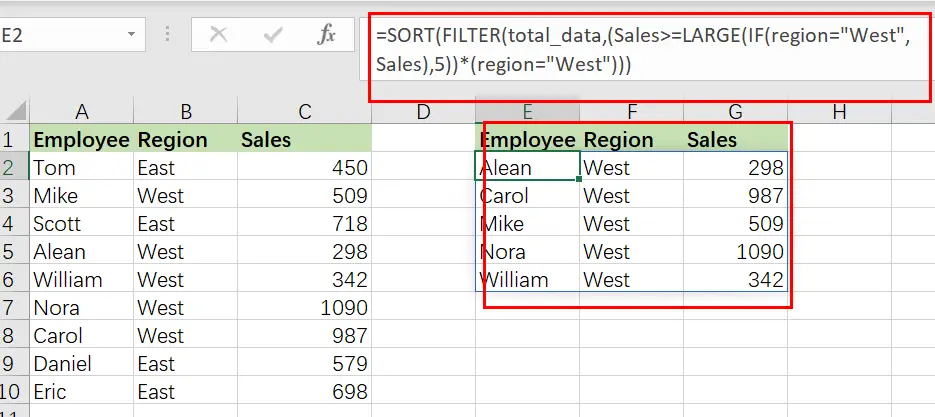
In this case, FILTER passes the results to the SORT function as an array parameter. The sort index is set to 3(sort results based on Sales values),while the sort order is set to -1 (descending order).

Related Functions

---

• Excel LARGE function
  The Excel LARGE function returns the largest numeric value from the numbers that you provided. Or returns the largest value in the array. The syntax of the LARGE function is as below:= LARGE (array,nth)…
• Excel IF function
  The Excel IF function perform a logical test to return one value if the condition is TRUE and return another value if the condition is FALSE. The IF function is a build-in function in Microsoft Excel and it is categorized as a Logical Function.The syntax of the IF function is as below:= IF (condition, [true_value], [false_value])….
• Excel Filter function
  The FILTER function extracts matched records from a collection of data using one or more logical checks. The include argument specifies logical tests, which might encompass a wide variety of formula conditions.==FILTER(array,include,[if empty])…
• Excel Sort function
  The SORT function in Excel sorts the contents of an array or range alphabetically or numerically by columns or rows.The syntax:=SORT(array, [sort index],) …