Just assume that you have a few cells containing values/words and you want to extract the last two words from each cell into another separate cell; then you might think that it’s not a big deal; because you would prefer to manually extract the last two words from the cell into another without any need of the formula then congratulations because you are thinking right, but let me add up that it would be a big deal to extract the last two words from the multiple cells to another cell and doing it manually would be a foolish attempt because you would get tired of it and would never complete your work on time.
But don’t be worry about it because after carefully reading this article, extracting last the two words from multiple cells into separate cells would become a piece of cake for you.
So let’s dive into the article to take you out of this fix.
Table of Contents
General formula:
The Following formula would help you out for extracting last the two words from multiple cells into separate cells :
=MID(B1,FIND("#",SUBSTITUTE(B1," ","#",LEN(B1)-LEN(SUBSTITUTE(B1," ",""))-1))+1,200)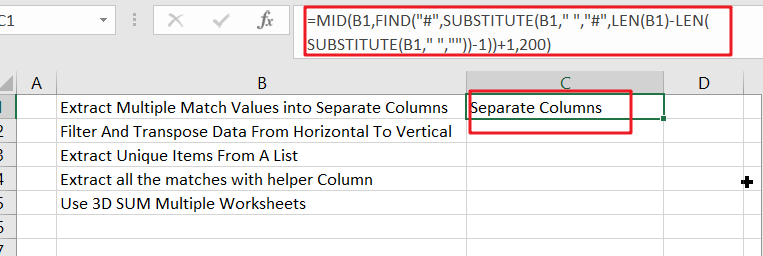
Syntax Explanations:
Before going into the explanation of the formula for getting the work done efficiently, we must understand each syntax which would make it easy for you that how each syntax contributes to extracting the last two words/values from multiple cells into separate cells:
MID: This function contributes to extracting the number or characters from the given string by starting from the left side.FIND: In Excel, this FIND function contributes to finding out one text inside the other one.LEN: In Excel, this LEN function contributes to finding out the length of the text string.SUBSTITUTE: In excel, this SUBSTITUTE function contributes to replacing the existing text with new text in a text string.- B1: this function represents the input value.
- Comma symbol (,): In Excel, this comma symbol acts as a separator that helps to separate a list of values.
- Parenthesis (): The core purpose of this Parenthesis symbol is to group the elements and to separate them from the rest of the elements.
- Minus Operator (-): This minus symbol contributes to subtracting any two values.
- Plus operator (+): This plus symbol adds the values.
Let’s See How This Formula Works:
The formula uses the MID function to extract the characters from the second to last space. The MID function accepts three arguments; the number of characters to extract, the starting position, the text to work with.
The text is from column B, and the number of characters can be large enough to ensure that the last two words are taken. The task is to figure out where to start, just after the second-to-last spot. The sophisticated work is mostly done with the SUBSTITUTE function, which accepts an optional input called instance number. This function is used to replace the second to last space in the text with the “#” character, which is then found using the FIND function.
The following snippet figures out how many total spaces are in the text, from which 1 is subtracted.
=LEN(B1)-LEN(SUBSTITUTE(B1," ","")-1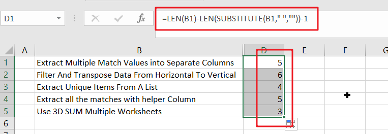
According to the example, the above code would return 5 because there are 6 spaces in the text. As the instance number, this returning number is then placed into the SUBSTITUTE function.
=SUBSTITUTE(B1," ","#",5)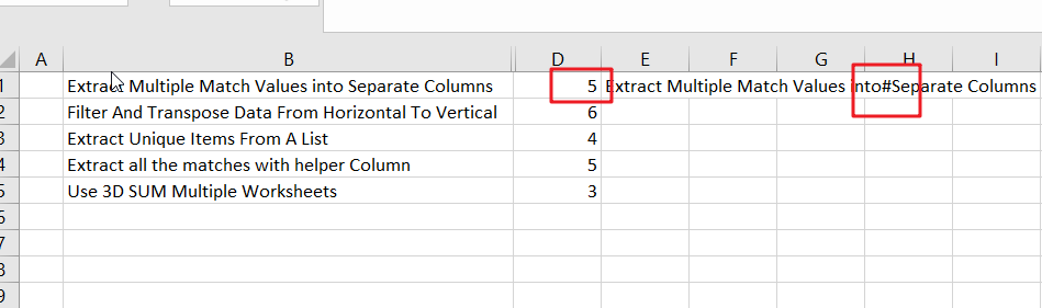
Due to the above placement of the returning number, the SUBSTITUTE function would replace the fifth space character with “#“, now you might be curious about it that why we are using “#” ? so here is the answer that it’s an arbitrary choice you can use any other character too but here is the condition that the chosen character would not appear in the original text.
After this, the FIND Function would locate the “#” character (or whatever character you would use) in the text:
=FIND("#","Extract Multiple Match Values into#Separate Columns")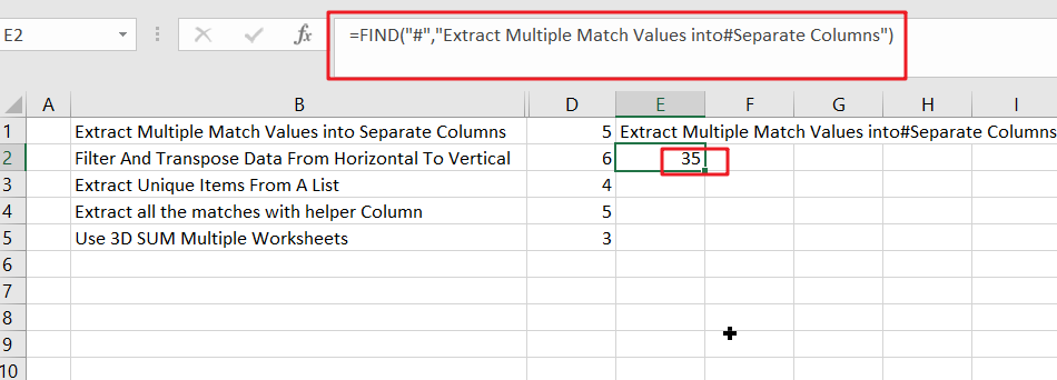 According to the example, the result of the FIND function would be 35, in which 1 is added for getting 36. This is the starting point, and as the second argument, it would go into the MID function.
2. Extract Last N words from String Using MID Function
In this formula, we have made the adjustments to extract the last 2 words from the cells and can also be generalized to extract the last N words from a cell by replacing the hardcoded 1 in the example with (N-1).
Moreover, if you want to extract many words, you must replace the hardcoded argument in MID, 200, with a larger number. To make sure that the number is large enough, you can use the LEN function, like it is used as follows:
=MID(B1,FIND("#",SUBSTITUTE(B1," ","#",LEN(B1)-LEN(SUBSTITUTE(B1," ",""))-1))+1,LEN(B1))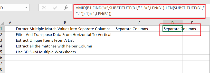
3. Extract Last N words from String using VBA Code
Let’s see the second method, we’ll leverage VBA to introduce a more dynamic and automated solution for extracting the last N words from a string in Excel.
For those seeking a programmatic approach, VBA provides a robust solution.
Open the Visual Basic for Applications editor by pressing ‘Alt + F11.’
Insert a new module and paste the following code:
Function ExtractLastNWords(inputString As String, n As Integer) As String
    Dim words() As String
    Dim resultString As String
    Dim i As Integer

    words = Split(inputString, " ")
    resultString = ""

    If n >= UBound(words) + 1 Then
        ExtractLastNWords = inputString
    Else
        For i = UBound(words) - n + 1 To UBound(words)
            resultString = resultString & words(i) & " "
        Next i
        ExtractLastNWords = Trim(resultString)
    End If
End Function
Save and close the editor.
Now, you can use this function in your worksheet, like this:
=ExtractLastNWords(B1, 3)where B1 is the cell containing your string, and 3 is the number of words you want to extract.
4. Video: Extract Last N words from String
This Excel video tutorial where we’ll unravel the secrets of extracting the last N words from a string. In this session, we’ll explore two distinct methods—utilizing a formula based on the MID function and employing VBA.
5. Related Functions
- Excel MID function
The Excel MID function returns a substring from a text string at the position that you specify.The syntax of the MID function is as below:= MID (text, start_num, num_chars)… - Excel Substitute function
The Excel SUBSTITUTE function replaces a new text string for an old text string in a text string. The syntax of the SUBSTITUTE function is as below:= SUBSTITUTE (text, old_text, new_text,[instance_num])…. - Excel LEN function
The Excel LEN function returns the length of a text string (the number of characters in a text string).The LEN function is a build-in function in Microsoft Excel and it is categorized as a Text Function.The syntax of the LEN function is as below:= LEN(text)… - Excel FIND function
The Excel FIND function returns the position of the first text string (sub string) within another text string.The syntax of the FIND function is as below:= FIND(find_text, within_text,[start_num])