This post will guide you how to use Excel TRUNC function with syntax and examples in Microsoft excel.

Description

The Excel TRUNC function truncates a number to an integer by removing the fractional part of the number. So this function returns a truncated number based on a given number of digits in Excel.

The TRUNC function is a build-in function in Microsoft Excel and it is categorized as a Math and Trigonometry Function.

The TRUNC function is available in Excel 2016, Excel 2013, Excel 2010, Excel 2007, Excel 2003, Excel XP, Excel 2000, Excel 2011 for Mac.

Syntax

The syntax of the TRUNC function is as below:

=TRUNC (number, number_digits)

Where the TRUNC function arguments are:

• number -This is a required argument. The number that you want to truncate.
• number_digits – This is an optional argument. It will specify the number of decimal places to truncate the given number to. If this argument is omitted, and the TRUNC function will set number_digits argument as zero value by default.

Note:

• If the number_digits argument is a positive value, the function will truncate the number of digits to the right of the decimal point.
• If the number_digits argument is equal to 0, then the function will truncate the number to the nearest integer.
• If the number_digits argument is a negative value, the function will truncate the number to the left of the decimal point.
• The TRUNC and INT functions are very similar, they both can return the integer part of a given number. The TRUNC function will remove the fractional part of the number. And the INT function will round numbers down to the nearest integer based on the value of the fractional part of the number. With negative number, the TRUNC function and the INT function are different, as the returned result are different.

Excel TRUNC Function Examples

The below examples will show you how to use Excel TRUNC Function to truncate a given number to a specified number of decimal places in Excel.

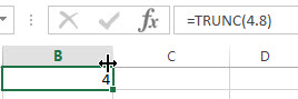
1# to truncate a number 4.8 to return the integer part, enter the following formula in Cell B1.

=TRUNC(4.8)

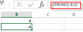
2# to truncate a negative number -4.5 to return the integer part, enter the following formula in Cell B2.

=TRUNC(-4.5)

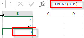
3# to truncate a number between 0 and 1 to return the integer part, enter the following formula in Cell B3.

=TRUNC(0.35)

---

Related Functions

• Excel INT Function
  The Excel INT function returns the integer portion of a given number. And it will rounds a given number down to the nearest integer. The syntax of the INT function is as below:= INT (number)…