This post will guide you how to use the PERCENTRANK function with syntax and examples in Microsoft excel.

Description

The Excel PERCENTRANK function returns the rank of a value in a set of values as a percentage of the set. So you can use the PERCENTRANK function to calculate the relative position of a value in a set of values as a percentage in Excel. This function has been replaced by the PERCENTRANK .INC function in Excel 2010.

The PERCENTRANK function is a build-in function in Microsoft Excel and it is categorized as a Statistical Function.

The PERCENTRANK function is available in Excel 2016, Excel 2013, Excel 2010, Excel 2007, Excel 2003, Excel XP, Excel 2000, Excel 2011 for Mac.

Syntax

The syntax of the PERCENTRANK function is as below:

= PERCENTRANK (array,x,[significance])

Where the PERCENTRANK function arguments are:

• Array – This is a required argument.  A range or array or cell reference from which you want to get the rank of a specific value.
• X – This is a required argument. The value that you want to find the rank for.
• Significance -This is an optional argument.  A value that identifies the number of significant digits for the returned percentage value. If omitted, PERCENTRANK uses three digits (0.xxx).

Note:

• If the array argument is empty, the PERCENTRANK function will return the #VALUE! Error.
• If the significance argument is small than 1, the PERCENTRANK function will return the #NUM! Error.
• If x does not match one of the values in the array, the PERCENTRANK function will interpolate to find the percentage rank.

Excel PERCENTRANK Function Examples

The below examples will show you how to use Excel PERCENTRANK Function to get the rank of a value in a data set as a percentage of the data set.

Example 1:  to get the percent rank of 3 in the range A1:A5, using the following formula:

= PERCENTRANK (A1:A5)

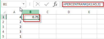
Because there are 3 values are less than 3, and 1 value is greater than 3, so the percent rank of 3 in the range A1:A5 is: 3/(3+1)=0.75

 

Example 2:  to get the percent rank of 4 in the range A1:A5, using the following formula:

= PERCENTRANK (A1:A5)

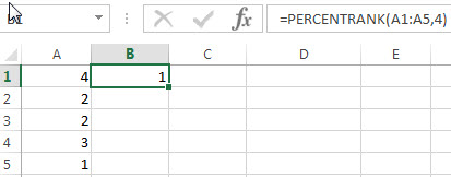
Because there are 4 values are less than 4, and 0 value is greater than 4, so the percent rank of 4 in the range A1:A5 is: 4/(4+0)=0.75