This post will guide you how to use the INTERCEPT function with syntax and examples in Microsoft excel.

Description

The Excel INTERCEPT function calculates the point at which a line will intersect the y-axis by using existing x-values and y-values. So it will return the y-axis intersection point of a line based on the existing x-axis values and y-axis values.

The INTERCEPT function is a build-in function in Microsoft Excel and it is categorized as a Statistical Function.

The INTERCEPT function is available in Excel 2016, Excel 2013, Excel 2010, Excel 2007, Excel 2003, Excel XP, Excel 2000, Excel 2011 for Mac.

Syntax

The syntax of the INTERCEPT function is as below:

=INTERCEPT (known_y's, known_x's)

Where the INTERCEPT function arguments are:

• known_y’s – This is a required argument.  The known y-values or range of data used to calculate the intersection.
• known_x’s -This is a required argument.  The known x-values or range of data used to calculate the intersection.

Note:

• The arguments should be numbers, or arrays, or references that contains only numeric values.
• If any array or reference argument contains text, logical values, or empty cells, the INTERCEPT function will ignore those values.
• If known_y’s and known_x’s arrays have a different lengths, or do not contain any values, the INTERCEPT function will return the #N/A Error.

Excel INTERCEPT Function Examples

The below examples will show you how to use Excel INTERCEPT Function to calculate the value at the intersection of the y-axis through a supplied set of x-values and y-values.

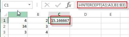
Example 1:   to calculate the point at which a line will intersect the y-axis by using the existing x-values A1:A3 and y-values B1:B3, using the following formula:

=INTERCEPT(A1:A3,B1:B3)