This post will guide you how to use Excel HLOOKUP function with syntax and examples in Microsoft excel.
Table of Contents
Description
The Excel HLOOKUP function lookup a value in the top row of the table and return the value in the same column based on index_num position.
The HLOOKUP function is a build-in function in Microsoft Excel and it is categorized as a Lookup and Reference Function.
The HLOOKUP function is available in Excel 2016, Excel 2013, Excel 2010, Excel 2007, Excel 2003, Excel XP, Excel 2000, Excel 2011 for Mac.
Syntax
The syntax of the HLOOKUP function is as below:
= HLOOKUP (lookup_value, table_array, row_index_num,[range_lookup])
Where the HLOOKUP function arguments are:
Lookup_value -This is a required argument. The value that you want to search for, in the first row of the table. Note: the lookup_value can be a value, a cell or ranges reference, or a text string.
Table_array – This is a required argument. Two or more rows of data to be searched in the top row.
Row_index_num – This is a required argument. The row number in table_array.
Range_lookup – This is a optional argument. The value can be set as True or False. If true, the function will return an approximate match value. If False, it will find an exact match or it will return an error value #N/A.
Example
The below examples will show you how to use Excel HLOOKUP Lookup and Reference Function.
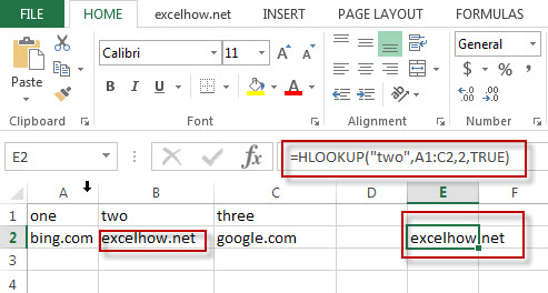
#1 To search “two” text string in row 1 and returns the value from row 2 that is in the same column, just using the following excel formula: =HLOOKUP(“two”,A1:C2,2,TRUE)
Leave a Reply
You must be logged in to post a comment.