This post will guide you how to highlight the date with different color using the conditional formatting feature in excel. How do I conditional formatting date with red, amber, or green color in excel. How to highlight the date with red if the cell dates is past now(). How to highlight the date with amber if the cell date is past now but within the next 6 months from now(). How to highlight the date with green if the cell date is more than 6 months from now.
Table of Contents
1. Conditional Formatting date with red Amber or Green
If you want to conditional formatting a list of date with different colors in excel, you just need to do the following steps:
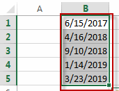
#1 select the date list in your worksheet
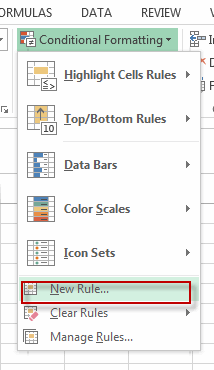
#2 go to HOME tab, click conditional Formatting command under Styles group. Then click New Rule…from the drop down list. The New Formatting Rule dialog will appear.
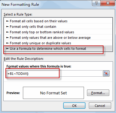
#3 click Use a formula to determine which cells to format in the section list of the Select a Rule Type. Then type this formula into the Format values where this formula is true text box. =B1<TODAY()
#4 click Format button, the Format Cells dialog will appear. Switch to Fill tab, select the red color.
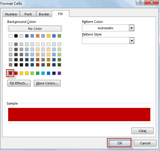
#5 click OK button. You will see that the past dates in the selected range are highlighted with red color.
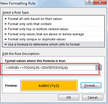
#6 To highlight the dates within the next 6 months from now, just use this formula =AND(B1>=TODAY(),B1<EDATE(TODAY(),6)) in the above step 3, then repeat the steps 4 and 5. Choose the Amber color in format Cells dialog.
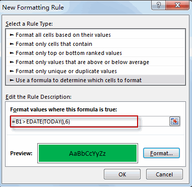
#7 to highlight the dates more than 6 months from now, just use this formula: =B1>EDATE(TODAY(),6) into the Format values where this formula is true text box in the above step 3. Then repeat the steps 4 and 5. Choose the green color in Format Cells dialog.
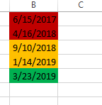
#8 Lets see the result:
2. Video: Conditional Formatting date with red Amber or Green
This tutorial video will guide you how to highlight the date with different color using the conditional formatting feature in excel.
3. SAMPLE FIlES
Below are sample files in Microsoft Excel that you can download for reference if you wish.
4. Related Functions
- Excel TODAY function
The Excel TODAY function returns the serial number of the current date. So you can get the current system date from the TODAY function. The syntax of the TODAY function is as below:=TODAY()… - Excel EDATE function
TThe Excel EDATE function returns the serial number that represents the date that is a specified number of months before or after a specified date.The syntax of the EDATE function is as below:=EDATE (start_date, months)… - Excel AND function
The Excel AND function returns TRUE if all of arguments are TRUE, and it returns FALSE if any of arguments are FALSE.The syntax of the AND function is as below:= AND (condition1,[condition2],…)…
Leave a Reply
You must be logged in to post a comment.