This post will guide you how to create drop-down list with color in Excel. How do I color coded a drop down list in Excel.

Color Coded Drop down List

---

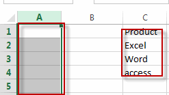
Assuming that you have a list of data that contain product name in range C1:C4, and you want to create a drop down list based on those data using Data Validation feature in excel. And then you still want to color coded this drop down list. How to achieve it. Let’s see the following detailed steps.

#1 select a range of cells that you want to put the drop down list in. such as: Column A.

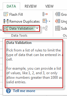
#2 go to DATA tab, click Data Validation command under Data Tools group. The Data Validation dialog will open.

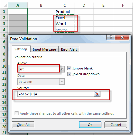
#3 select List from the Allow list box, and click Source button to select the source values that you want to add into the drop list.

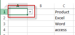
#4 click OK button. You will see that a newly drop down list has been created in selected column A.

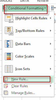
#5 select the column A, go to HOME tab, click Conditional Formatting command under Styles group. And select New Rule from the drop down menu list. The New Formatting Rule will open.

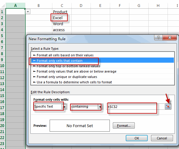
#6 select Format only cells that contain from the Select a Rule Type section. And in Format only cells with section, select Specific Text in the first drop-down list box, select containing in the second drop-down list box, and click the source button in the third text box to select one value that you want to be colored.

#7 click Format button, the Format cells dialog will open. And switch to Fill tab, select one color that you want to set. Click OK button.

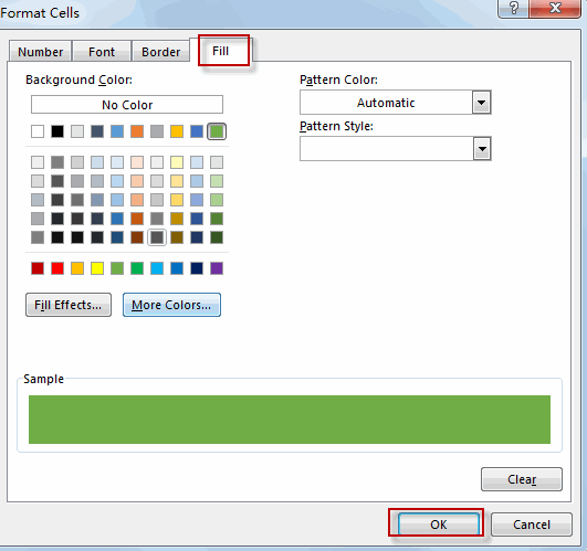
#8 click OK button again.

#9 you can repeat the above steps 5 to 8 for other values in the drop down list.

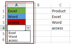
#10 let’s see the last result.