Are you weary of investing a lot of time and effort in manually calculating the average of the numbers by including or excluding 0 and calculating the average of the top 3 scores? Then congratulations because you have just landed on the right article.
In this article, you will get to know the smarter ways to do these cumbersome tasks in a matter of seconds.
So without any delay, let’s dive into the article,
Table of Contents
Average Of The Numbers By Including 0
General Formula
Use the formula below to calculate the average of a set of numbers in Excel:
=AVERAGE(range)
Explanations for Syntax:
-
AVERAGE: In Excel, the AVERAGE Function can calculate the arithmetic mean of a set of numbers. Range: This is the input value from your worksheet.Comma symbol (,):It acts as a separator that helps to separate a list of values.Parenthesis (): The main Function of this symbol is to group the elements.
Explanation
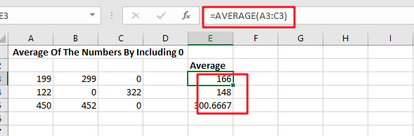
Use the AVERAGE function to calculate the average of a set of numbers.
In the example, the formula in E3 is:
=AVERAGE(A3:C3)
which is then copied down in the table.
AVERAGE is a built-in function in MS Excel in which you supply a range of cells to average, and this function returns the result. In cases where cells are not adjacent, you can also provide individual arguments to the Function.
The AVERAGE function automatically ignores all the blank text and cells, but zero values are included.
Average Of The Numbers By Ignoring 0
General Formula
The formula below will assist you in calculating the average of a number that excludes zero:
=AVERAGEIF(range,"<>0")
Explanations for Syntax:
AVERAGEIF: This Function returns the average of a set of input values that satisfy a single condition or criteria. Learn more about the AVERAGEIF Function.
Range: This is the input value from your worksheet.
Comma symbol (,): It acts as a separator that helps to separate a list of values.
Parenthesis (): The main Function of this symbol is to group the elements.
Operator (>): The supplied criteria is “>0,” which means “not equal to zero.”
Explanation
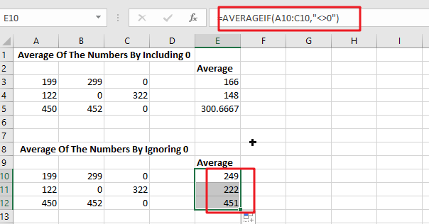
The AVERAGEIF function computes the average of a set of numbers while excluding or ignoring zero values. In the example, the formula in E10 is:
=AVERAGEIF(A10:C10,"<>0")
The formula in E3 in the example is based on the AVERAGE Function:
=AVERAGE(A3:C3)
Because (129+299+0)/ 3 = 166, the answer is 166.
To remove the zero from the calculated average, the formula in E10 employs the AVERAGEIF function, as shown below:
=AVERAGEIF(A10:C10,"<>0") / returns 249
The provided criterion is “>0,” which means “not equal to zero”.
Data with no values
Because the AVERAGE, AVERAGEIF, and AVERAGEIFS functions all ignore blank cells (and cells with text values), there isn’t any need to provide criteria to filter out empty cells.
Average Of The Top 3 Numbers
General Formula
The formula below will assist you in calculating the average of the top 3 numbers:
=AVERAGE(LARGE(range,{1,2,3}))
Explanations for Syntax:
AVERAGE:In Excel, the AVERAGE Function can calculate the arithmetic mean of a set of numbers.Range:This is the input value from your worksheet.Comma symbol (,): It acts as a separator that helps to separate a list of values.Parenthesis (): The main Function of this symbol is to group the elements.LARGE:This Function returns the Nth largest value from the given range of data. Learn more about the LARGE Function.Values:This is the range of cells that contain values.
Explanation
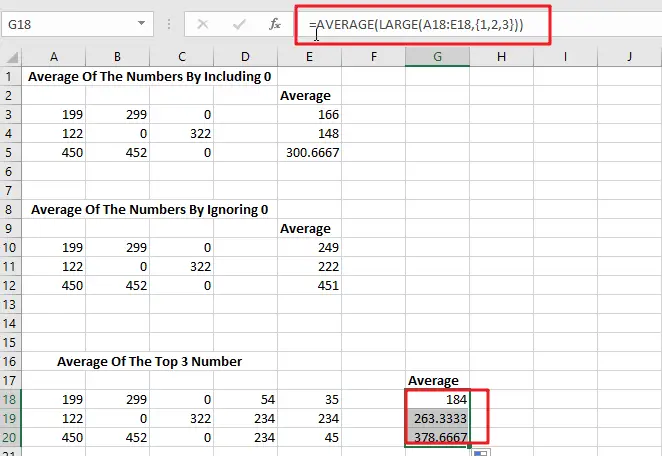
To average the top three values in a data set, use a formula based on the LARGE and AVERAGE functions. In this example, the formula in G18 is mentioned below:
=AVERAGE(LARGE(A18:E18,{1,2,3}))
The LARGE function is used to find the top nth value in a set of numbers. For example, the LARGE(A18:E18,{1,2,3})will return the highest value, LARGE(A18:E18,2) will return the second-highest value, and so on:
=LARGE(A18:E18,1)/ First largest value
=LARGE(A18:E18,2)/ 2nd largest value
=LARGE(A18:E18,3)/ 2nd largest value
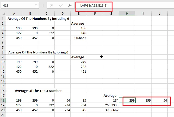
In this case, we are requesting multiple values by passing an array constant 1,2,3 into LARGE as the second argument. This causes LARGE to return an array of the top three values.
=LARGE(A18:E18,{1,2,3})
returns an array similar to this:
{299,199,54}
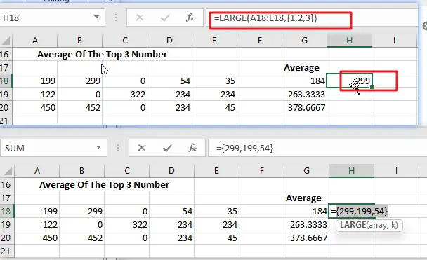
This array is passed directly to the AVERAGE function:
=AVERAGE(299,199,54) / returns 184
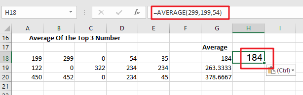
The AVERAGE Function then returns the average of these values.
Because the AVERAGE Function can handle arrays natively, there is no need to enter this formula with control + shift + enter.
Related Functions
- Excel AVERAGE function
The Excel AVERAGE function returns the average of the numbers that you provided.The syntax of the AVERAGE function is as below:=AVERAGE (number1,[number2],…)…. - Excel AVERAGEIF function
The Excel AVERAGEAIF function returns the average of all numbers in a range of cells that meet a given criteria.The syntax of the AVERAGEIF function is as below:= AVERAGEIF (range, criteria, [average_range])…. - Excel LARGE function
The Excel LARGE function returns the largest numeric value from the numbers that you provided. Or returns the largest value in the array. The syntax of the LARGE function is as below:= LARGE (array,nth)…