Assume that you have been assigned a task of calculating the average response time per month in MS Excel, then; if you are new to MS Excel, doing this task manually might be your first attempt which would not only make you tired, but you won’t complete your work on time.

But fortunately, there is a more innovative way by which you can do this cumbersome task in a matter of seconds, so kindly read this article till the end and let’s dive into it,

General Formula:

Use the formula below to calculate the average time per month in Excel.

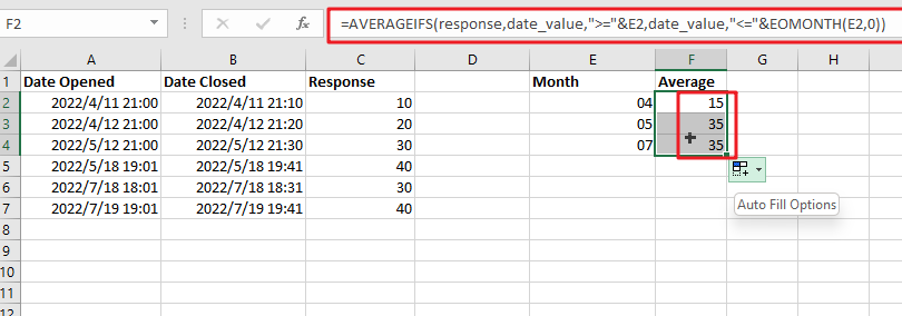
=AVERAGEIFS(response,date_value,">="&E2,date_value,"<="&EOMONTH(E2,0))

Explanations for Syntax:

• AVERAGEIFS: This Function returns the average of a set of input values that meet multiple criteria. Learn more about the AVERAGEIFS Function.
• EOMONTH: In Excel, the EOMONTH Function can be used to return the last day of the month after adding or subtracting a specified number of months from a date.
• Response: The response is calculated by subtracting the date opened from the date closed.
• Date_value: These are the input dates from your worksheet.
• Criteria (E2): It specifies the month used to calculate the average.

 Explanation

To average response times by month, use a formula based on the AVERAGEIFS and EOMONTH Functions.

In the example, the formula in F2 is mentioned below:

=AVERAGEIFS(response,date_value,">="&E2,date_value,"<="&EOMONTH(E2,0))

This formula employs the named ranges “ date_value ” (A2:A7) and “ response ” (C2:C7). Column C’s response are in minutes and are calculated by subtracting the date opened from the date closed.

The AVERAGEIFS function is intended to average ranges based on multiple criteria; that’s why we would configure the AVERAGEIFS process to average durations by month based on two criteria:

1^st criteria are in which the matching dates are either greater than or equal to the first day of the month, and the 2^nd  criteria are in which the matching dates are either less than or equal to the last day of the month.

In column E, we just type month names, such as: 04,05,07.

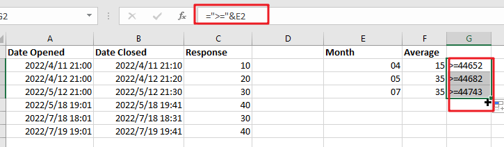
This makes it easier to create the AVERAGEIFS function’s criteria we need by using the values in the F column. To match that either the dates greater than or equal to the four of the month, we use:

">="&E2

To match dates that are less than or equal to the last day of the month, we use:

"<="&EOMONTH(E2,0)

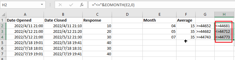
By providing zero for the month’s argument, we can get the EOMONTH to return on the last day of the same month.

When the building criteria are based on a cell reference, oncatenation with an ampersand (&) is required.

So we know that using the formula mentioned above, you can obtain the average response times by month. This tutorial will learn how to calculate the average monthly response time in a Microsoft Excel workbook. As we know, the AVERAGEIFS Function is intended to average ranges based on multiple criteria. In the following example, we configure AVERAGEIFS to average durations by month using two criteria: first, we match dates greater than or equal to the first day of the month. Second, by matching dates less than or equal to the last day of the month. So, using this formula, you can obtain the average response time per month in the workbook in Microsoft Excel.

Pivot Table

When you need to summarise or average data by year, month, quarter, and so on, then a pivot table is an excellent solution because pivot tables automatically group dates.

Related Functions

• Excel AVERAGEIFS function
  The Excel AVERAGEAIFS function returns the average of all numbers in a range of cells that meet multiple criteria.The syntax of the AVERAGEIFS function is as below:= AVERAGEIFS (average_range, criteria_range1, criteria1, [criteria_range2, criteria2],…)….