You might have come across a task in which you were assigned to build hyperlinks, which seems very easy, and if you are new to excel or don’t have enough experience with it, then you might wonder about doing this task manually but let me add that no doubt it seems easy to build two or three hyperlinks manually, but when it comes to building a bulk of hyperlinks, then it becomes a cumbersome task to do it manually moreover you will end up exhausted, and you might not finish the task on time.
But don’t worry about it because we got your back and brought up the easiest way, which is none other than with the aid of the Vlookup Function, which lets you build bulks of hyperlinks within seconds.
So without any delay, let’s dive into it
Table of Contents
General Formula
To create hyperlinks using VLOOKUP, use the formula below.
=HYPERLINK(VLOOKUP(Lookup_name,Lookup_range,column_number,0), Lookup_name)
Explanation Of Syntax
- Hyperlink: The HYPERLINK function creates a clickable hyperlink. This Function can develop connections to workbook locations, internet sites, or files on network servers.
- VLOOKUP: This Function helps lookup data in a range or table row by row. More information on the VLOOKUP function may be found here.
- The comma symbol (,): This symbol is a separator that aids in the separation of a list of values.
- Parenthesis (): This symbol’s Primary Function is to group the elements.
Summary
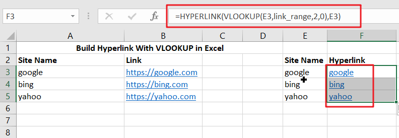
You may use the VLOOKUP function in conjunction with the HYPERLINK function to produce a hyperlink from a lookup.
The formula in F5 in the case provided is:
=HYPERLINK(VLOOKUP(E3,link_range,2,0),E3)
Explanation
The hyperlink function allows you to use a formula to build a functioning link. It accepts two parameters: link location and, optionally, familiar name.
VLOOKUP searches for and obtains a link value from column 2 of the designated range “link_range” from the inside out (A3:B5). The lookup value is taken from column E, and VLOOKUP is set to an exact match.
The result is used as link location in HYPERLINK, while column E’s content is used as a friendly name.
HYPERLINK function returns a functional link.
As an example,
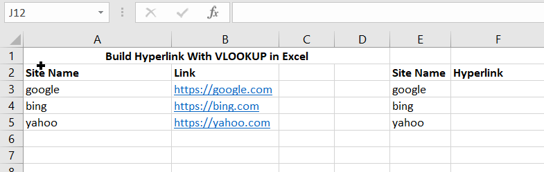
To create hyperlinks in Excel using VLOOKUP, follow the instructions below.
- To begin, you must prepare sample data in Excel.
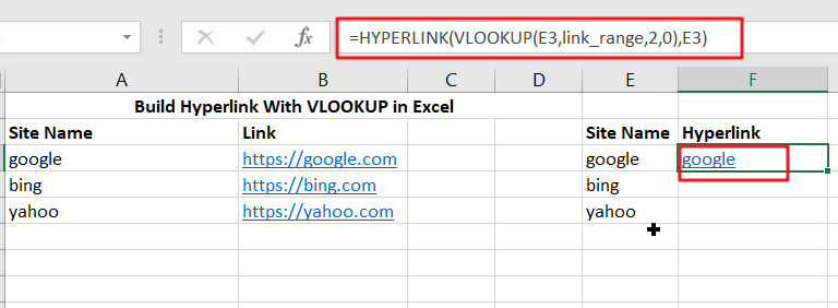
- Then, insert the following formula in the formula bar to create a hyperlink from a lookup. Use the Formula
=HYPERLINK(VLOOKUP(E3,link_range,2,0),E3)
- To obtain the result, press the Enter key, as illustrated in cell F3.
- Next, insert the following formula in the formula bar to create a hyperlink from a lookup. Use the Formula
=HYPERLINK(VLOOKUP(E4,link_range,2,0),E4)
- Finally, press the Enter key to obtain the result, as shown in cell F4 below.
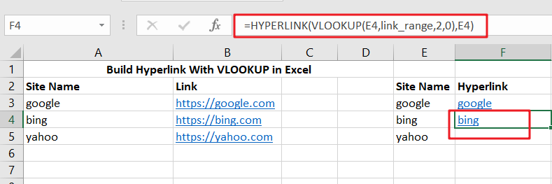
Cell F4, as a result
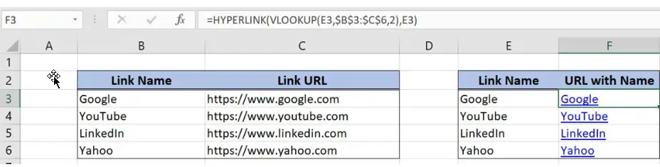
In another example, we want to retrieve the Link URL from column C based on the Link Name in E3 (Google). We want to build a hyperlink with a name based on those two variables. The outcome is shown in cell F3.
The equation is as follows:
=HYPERLINK(VLOOKUP(E3, $B$3:$C$6, 2), E3)
Cell E3 contains the lookup value. The table array argument has the value range $B$3:$C$6. Because the range does not change when the formula is duplicated, it must be fixed. Col index num is set to 2, indicating that we want to get data from the second column in the range. Finally, the default value for range lookup is 0 since we want to discover an exact match of “Lookup column” values.
The link location parameter for the HYPERLINK function is the result of the VLOOKUP function. Cell E3 is the friendly name parameter.
To use the HYPERLINK and VLOOKUP capabilities, we must first do the following steps:
Step1: Click on cell F3 to insert the formula:
=HYPERLINK(VLOOKUP(E3, $B$3:$C$6, 2), E3)
Step2: Enter the formula
Step3: Drag the formula down to the remaining cells in the column by clicking and dragging the small “+” button at the bottom-right of the cell.
Use of the self-contained VLOOKUP formula
Consequently, the hyperlink for https://www.google.com with the name “Google” will appear in cell F3. The VLOOKUP table shows that this is the Link URL for the term Google from E3.
Conclusion
This article will teach you to efficiently create hyperlinks using VLOOKUP in MS Excel with examples and pictures.
Related Functions
- Excel HYPERLINK function
The Excel HYPERLINK function creates a shortcut/hyperlink to a document, when you click this hyperlink, the excel will open the file that is stored on a network server or local location.The syntax of the HYPERLINK function is as below:= HYPERLINK(link_location,[friendly_name])… - Excel VLOOKUP function
The Excel VLOOKUP function lookup a value in the first column of the table and return the value in the same row based on index_num position.The syntax of the VLOOKUP function is as below:= VLOOKUP (lookup_value, table_array, column_index_num,[range_lookup])….