AVERAGE function is one of the most popular functions in Excel. Apply AVERAGE together with some other functions, we can calculate average properly based on different situations.

In this article, we will introduce you the way to calculate average of the top N numbers from a range. To approach our goal, except the main AVERAGE function, we also apply LARGE function.

EXAMPLE

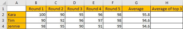
In this case, we want to calculate the average of the top three scores from 5-rounds competitions for each student. To calculate the average of top N values, we need the help of LARGE function.

SOLUTION

To create a formula to get average in this case, we need to know:

1) Find out the top three values by LARGE function.

2) Calculate average of the top three values by AVERAGE function.

The general formula is =AVERAGE(LARGE(Range,{1,2,…,N})).

FORMULA with AVERAGE & OTHER FUNCTIONS

In C2, we input the formula =AVERAGE(LARGE(B2:F2,{1,2,3})). After typing, press Enter, then average “98” of the top three scores is returned.

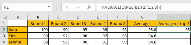
For Kara, five scores are saved in range B2:F2, the top three values are 100, 96 and 98, so the average is (100+96+98)/3=98, the formula returns correct result.

FUNCTION INTRODUCTION

The main function in this formula is “AVERAGE”, it returns the average of the top three values by our demands; “LARGE” is used for searching for the top three values among all given values.

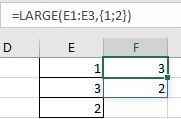
 a. LARGE function returns the Kth largest number from a given set of numbers or a range reference.

Syntax:

=LARGE(array,k)

 Example:

//If we input 2 for, only the second top value is returned;

//If we want to returning more than one top value, we can set an array constant as the function’s second argument;

//If we input {1;2} for k, 1 and 2 are separated by “;”, the top two values are saved in the same column;

//If we input {1,2} for k, 1 and 2 are separated by “,”, the top two values are saved in the same row.

 

b. AVERAGE function returns the average of numbers from a given range reference.

Syntax:

=AVERAGE(number1, [number2], …)

 

Example:

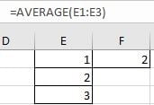
//For arguments “number1, number2,…”, they can be a set of numbers, or an array of numbers like {1;2;3}.

 FORMULA EXPLANATION

=AVERAGE(LARGE(B2:F2,{1,2,3}))

//This formula contains 2 functions, we explain functions from inside to outside.

a. For LARGE(B2:F2,{1,2,3}), range B2:F2 provides all scores from 5 rounds competitions; array constant {1,2,3} is the second argument “k” value, it determines the count of top numbers returned by LARGE.

In this case, B2:F2 is {}, LARGE returns below array:

LARGE({100,90,95,96,98},{1,2,3}) -> {100,98,96}

b. Array {100,98,96} from last step goes into AVERAGE calculation now.

=AVERAGE({100,98,96})

So, we get 98 properly after above two steps.

Related Functions

---

• Excel AVERAGE function
  The Excel AVERAGE function returns the average of the numbers that you provided.The syntax of the AVERAGE function is as below:=AVERAGE (number1,[number2],…)….
• Excel LARGE function
  The Excel LARGE function returns the largest numeric value from the numbers that you provided. Or returns the largest value in the array. The syntax of the LARGE function is as below:= LARGE (array,nth)…