Have you ever come across a task to calculate the average of the numbers with respect to multiple criteria? Are you tired of doing this cumbersome task manually? Are you willing to do this task smartly in just a matter of seconds? Then congratulations because you have just landed on the right article.
In this article, you will get to know the easiest way to calculate the average of the numbers with respect to multiple criteria in no time.
So read this article till the end, and let’s dive into it;
General Formula
=AVERAGEIFS(values,range1,criteria1,range2,criteria2)
Explanations for Syntax:
Before learning how to use the above formula, let’s first understand the role of each syntax in quickly calculating the average of the numbers concerning multiple criteria.
AVERAGEIFS: In Excel, this function returns the average of a set of input values that meet multiple criteria. Learn more about the AVERAGEIFS Function.Comma symbol(,): It acts as a separator that helps to separate a list of values.Parenthesis(): The main function of this symbol is to group the elements.Range: It represents the input value from your worksheet.Criteria: The specific criteria or values used to calculate the average.
Explanation
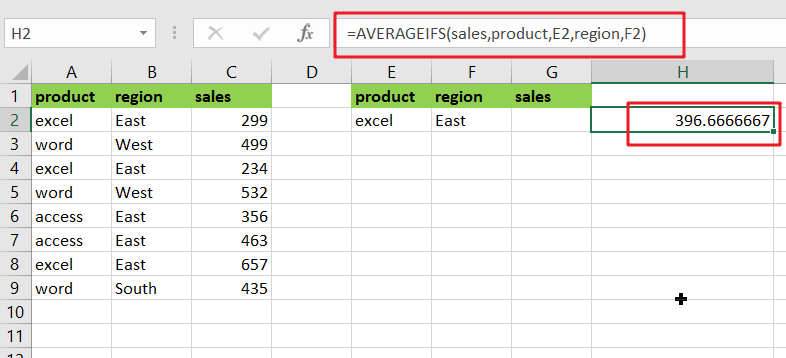
You can use the AVERAGEIFS function to average numbers based on multiple criteria. In the example, the formula in H2 is as follows:
=AVERAGEIFS(sales,product,E2,region,F2)
Where “sales” (C2:C9), “product” (A2:A9), and “sales” (C2:C9) are named ranges.
The AVERAGEIFS function, like the COUNTIFS and SUMIFS functions, is intended to handle multiple criteria that are entered in [range, criteria] pairs. AVERAGEIFS’s behavior is fully automatic as long as this information is provided correctly.
In the example, we have product values in column E and region values in column F. We use these values directly by using cell references as criteria.
The first argument holds the range of values to average:sales range
To limit the calculation by product, we provide:product, E2
We use the following formula to limit the calculation by region:region, F2
The answer in cell H2 is 396:
Now, let’s go to the 2nd example in which we want to average the product of “excel” and the sales greater than 300. Please follow these instructions:
Enter the formula given below into a blank cell:
=AVERAGEIFS(sales,product,E2,sales,F2)
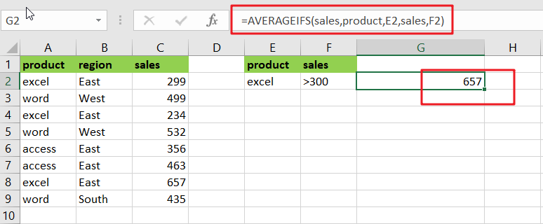
(product range is the data that contains the criteria1, sales range is the range which we want to calculate the average, E2 and F2 are the criteria1 and criteria 2), then press the Enter key to get the desired result. Take a look at this screenshot:
Note: If you need more than two criteria, add the criteria ranges and criteria you require as follows:
=AVERAGEIFS(sales,product,E2,region,F2,sales,G2)
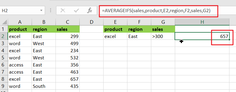
Note: the first criteria range is product and E2, the second criteria range is region and F2 and the third criteria is sales and G2 and the range you want to average the values is the criteria, sales range.
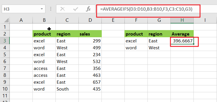
For Better understanding, we are adding up the 3rd example as follows:
- Consider the example below to calculate the average of numbers based on multiple criteria.
- The image below will show the input values for Columns B, C, and D.
- Next, enter the given formula in the formula bar section.
- Finally, we’ll see the result in cell H3.
Summary
This article explains how to use the formulas in Excel to calculate the average of numbers with multiple criteria. I hope you found this article interesting. If you have any ideas, please share them with us.
Related Functions
- Excel AVERAGEIFS function
The Excel AVERAGEAIFS function returns the average of all numbers in a range of cells that meet multiple criteria.The syntax of the AVERAGEIFS function is as below:= AVERAGEIFS (average_range, criteria_range1, criteria1, [criteria_range2, criteria2],…)…. - Excel COUNTIFS function
The Excel COUNTIFS function returns the count of cells in a range that meet one or more criteria. The syntax of the COUNTIFS function is as below:= COUNTIFS(criteria_range1, criteria1, [criteria_range2, criteria2]…)… - Excel SUMIFS Function
The Excel SUMIFS function sum the numbers in the range of cells that meet a single or multiple criteria that you specify. The syntax of the SUMIFS function is as below:=SUMIFS (sum_range, criteria_range1, criteria1, [criteria_range2, criteria2], …)…