Average is a valuable function in Excel that allows you to rapidly compute the average of the past N values in a column. However, you may need to insert new numbers beneath your original information from time to time, and you just want the average result to be updated automatically when new data is entered. This means you would like the average to always represent the latest N values in your data list, regardless of whether or not you add new data points.

The Generic formula is as follow:

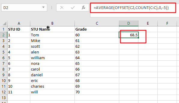
=AVERAGE(OFFSET(C2,COUNT(C:C),0,-N_Values))

Summary 

The AVERAGE function, in conjunction with the COUNT and OFFSET functions, may be used to calculate an average of the latest 5 data points. You may use this strategy to average the most recent N data points, such as the most recent 3 days, the most recent 6 measures, and so on. The following is the formula in D2 in the case shown:

=AVERAGE(OFFSET(C3,COUNT(C:C),0,-5))

Let’s See How This Formula Works

This function may be used to create dynamic rectangular ranges using a beginning reference and the values of the rows, columns, height, and width parameters. The rows and columns parameters are treated as “offsets” from the initial reference in the same manner. The number of rows and columns in the final range is determined by the height and width parameters (both of which are optional). For the sake of this example, OFFSET is set as follows:

• reference = C2
• rows = COUNT(C:C)
• cols = 0
• height = -5
• width = (not provided)

The beginning reference is supplied as C2, which is the cell immediately above the actual data in the table. Because we want OFFSET to provide a range of values starting with the last item in column C. We use the COUNT function to count all of the values in column C to get the needed row offset for OFFSET. COUNT solely counts numeric numbers, which means that the heading in row 1 is discarded automatically.

OFFSET resolves to the following when there are 10 numerical values in column C:

=OFFSET(C3,11,0,-5)

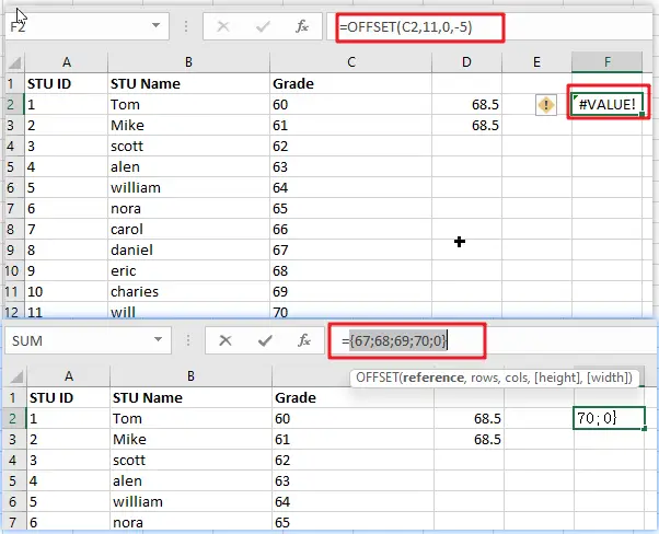
This combination of parameters begins at C2, offsets 11 rows to C12, and then uses -5 to expand the rectangular range up “backwards” 5 rows to form the range C8:C12, which is the range C2:C12.

At the end of the process, the OFFSET function passes the range C8:C12 to the AVERAGE function, which computes the average values in the range.

With a dynamic range

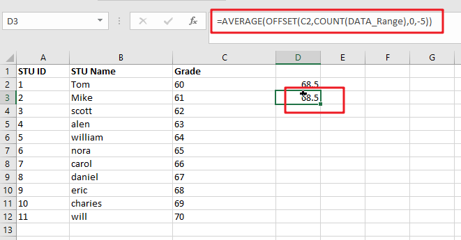
For the sake of simplicity, the example in this section utilises a complete column reference for the data that is being averaged – when new information is added to column C. The formula will continue to function correctly since reference C includes the whole column C. However, you may also utilise a dynamic range in the following manner:

=AVERAGE(OFFSET(C3,COUNT(DATA_Range),0,-5))

Where ” DATA_Range ” refers to a dynamic named range or a reference to a column in an Excel Table, respectively. Excel Tables and dynamic named ranges can dynamically expand as new data is entered, which is crucial for using this method. Take note that the reference to OFFSET is still in the row before the data appears.

Related Functions

---

• Excel AVERAGE function
  The Excel AVERAGE function returns the average of the numbers that you provided.The syntax of the AVERAGE function is as below:=AVERAGE (number1,[number2],…)….
• Excel COUNT function
  The Excel COUNT function counts the number of cells that contain numbers, and counts numbers within the list of arguments. It returns a numeric value that indicate the number of cells that contain numbers in a range…