In our daily work, we often encounter the situation of finding data based on the original data and conditions provided, such as finding cell phone numbers based on name, finding employee names and positions based on HRID, etc.
When we talk about the lookup function in excel workbook, most people will first think of using the VLOOKUP function. VLOOKUP function is the most commonly used lookup function in excel, even if you don’t use VLOOKUP function, you must have heard of it. How do we apply the VLOOKUP function in excel? What can it help us to achieve? Can we do lookups across worksheets? Today we will discuss the applications and usages of VLOOKUP function in Microsoft Excel Spreadsheet.
Whether you’re a beginner or have some experience with Excel, this step by step VLOOKUP function tutorial is an essential resource for improving your data analysis skills.
Table of Contents
- What is VLOOKUP Function in Excel
- Where is VLOOKUP Function in Excel
- How To Use VLOOKUP Function & Formula
- VLOOKUP Function Examples
- 11. How To Do a VLOOKUP with an IF Function
- 12. How To Use VLOOKUP with AND Function
- 13. VLOOKUP Function with & Operator
- 14. VLOOKUP Function with CHOOSE Function
- 15. VLOOKUP Exact Match
- 16. VLOOKUP Approximate Match
- 17. VLOOKUP with Absolute Range Reference
- 18. VLOOKUP with Duplicate Lookup Value
- 19. VLOOKUP Lookup the Largest/Smallest value
- 20. VLOOKUP Reverse Lookup
- 21. VLOOKUP to Return Multiple Values
- 22. VLOOKUP to Return Multiple Column Values
- 23. VLOOKUP Two-Conditional Lookup
- 24. VLOOKUP with Wildcards
- 25. VLOOKUP Range Lookup by Approximate Match
- VLOOKUP Error Value Handling
What is VLOOKUP Function in Excel
1. VLOOKUP Function Definition
The VLOOKUP function in Microsoft Excel is a built-in formula used to search for a specific value in the first column of a table array and return a related value from another column in the same row. It stands for Vertical Lookup, as the function searches for the value vertically in the first column of the table array.
If you need to find data by column, you need to use the HLOOKUP function, which is a horizontal lookup function with the similar arguments and usage as the VLOOKUP function.
The VLOOKUP function is not case sensitive. It treats upper-case and lower-case characters as the same and returns a match regardless of the case of the search value or the values in the first column of the table array.
The VLOOKUP function is available in Microsoft Excel 365, Excel 2019, Excel 2016, Excel 2013 and Excel 2010.
2. Two Types of VLOOKUP functions
There are two types of VLOOKUP functions in Microsoft Excel:
- Exact Match VLOOKUP: Returns the exact match for the search value, if it exists in the first column of the table array. It returns an error if the exact match is not found.
- Approximate Match VLOOKUP: Returns the closest match for the search value, based on the closest value that is less than or equal to the search value.
If you want to use the approximate match VLOOKUP, just set the last (optional) argument to TRUE or omit it, while to use the exact match VLOOKUP, you need to set the last argument to FALSE.
3. Limitations of VLOOKUP Function
The VLOOKUP function has the following limitations in MS Excel Spreadsheet:
- Can only search the first column: The VLOOKUP function can only search for a value in the first column of the specified table array, which limits its use in certain scenarios where values may be located in other columns.
- Only returns the first match: If there are multiple instances of the lookup value in the first column, the VLOOKUP function will only return the first match, not all of them.
- Can only return values from the same row: The VLOOKUP function can only return values from the same row as the lookup value, not from different rows or columns.
- Can only return values to the right: The VLOOKUP function can only return values that are located to the right of the lookup value in the same row, not values to the left.
- Can be slow with large data sets: The VLOOKUP function may slow down your spreadsheet if used extensively on large data sets, as it recalculates every time the worksheet is calculated.
Despite these limitations, the VLOOKUP function is still a widely used and valuable tool in Microsoft Excel, particularly for basic data analysis and retrieval tasks. To overcome these limitations, you may consider using other functions such as INDEX and MATCH, or using arrays and conditional statements in combination with VLOOKUP.
Where is VLOOKUP Function in Excel
The VLOOKUP function can be found in Microsoft Excel in the “Formulas” ribbon or Formula box.
4. Insert VLOOKUP Function Using Formulas Ribbon
The following are the steps to insert the VLOOKUP function in Microsoft Excel spreadsheets using the Formulas ribbon.
Step 1: Select the cell where you want the result of the VLOOKUP function to be displayed.
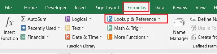
Step 2: Go to the “Formulas” ribbon and click on the “Lookup & Reference” category.
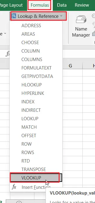
Step 3: From the “Lookup & Reference” category, click on the “VLOOKUP” function.
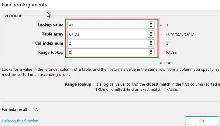
Step 4: The VLOOKUP function will be inserted into the selected cell and the Function argument dialog box will appear.
Step 5: In the Function argument dialog box, specify the following values for each of the VLOOKUP function’s arguments: Lookup Value, Table Array, col_index_num, [Range Lookup].
Step 6: Press “Enter” or click “OK” to complete the function and display the result in the selected cell.
5. Insert VLOOKUP Function in the Formula Box
The following are the steps to insert the VLOOKUP function in Microsoft Excel spreadsheets using the Formula box:
Step 1: Select the cell where you want the result of the VLOOKUP function to be displayed.
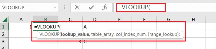
Step 2:Type “=VLOOKUP(” in the formula box.
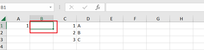
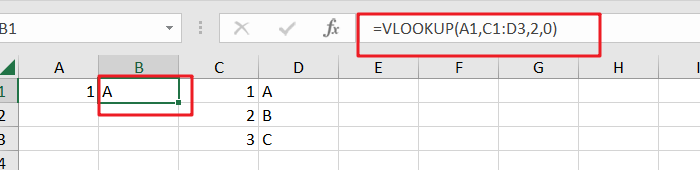
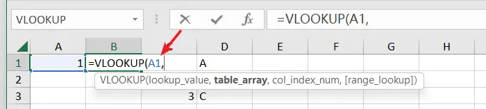
Step 3: Specify the lookup value in the first argument. For example, you can type a cell reference, such as “A1“, or a value in quotes, such as “A“.
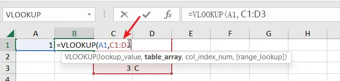
Step 4: Type a comma to move to the next argument, which is the table array. For example, you can type “C1:D3” to specify a range of cells from C1 to D3 as the table array.
Step 5: Type a comma to move to the next argument, which is the column index number. For example, you can type “2” to specify that you want to return the value from the second column in the table array.
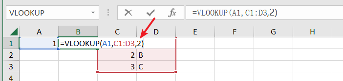
Step 6: Type “)” to close the function.
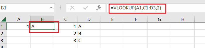
Step 7: Press “Enter” to complete the function and display the result in the selected cell.
How To Use VLOOKUP Function & Formula
The VLOOKUP function can be confusing at first, but with practice and understanding of the function’s syntax and arguments, it can be a useful function.The below is a brief explanation on how to use the VLOOKUP function in Microsoft Excel Spreadsheet.
6. VLOOKUP Function Syntax and Arguments
The correct syntax of VLOOKUP function is as below:
=VLOOKUP(lookup_value,table_array,col_index_num,[range_lookup])| Argument | Description | Data Type |
| lookup_value | Value to find | A numeric value, reference or text string |
| table_array | Lookup area | Data table |
| index_num | Returns the number of columns in the lookup area | Integer (positive) |
| range_lookup | Exact match / Approximate match | False (0, exact match) True (1 or empty, approximate match) |
4 arguments of VLOOKUP function are explained as follows:
- lookup_value is the value to be looked up, which appears in the first column of the data table. lookup_value can be a numeric value, a cell or area reference, a text string. When this parameter is omitted, it means that look up is performed with 0 value.
- table_array is the data table to look for. Enter a cell or range reference or table name.
- col_index_num is the data column number of the table_array. col_index_num is 1, the value of the first column of the table_array is returned, col_index_num is 2, the value of the second column of the table_array is returned. If col_index_num is less than 1, VLOOKUP returns the error value #VALUE!, if col_index_num is greater than the number of columns of table_array, VLOOKUP returns the error value #REF!.
- range_lookup is a logical value that specifies whether the VLOOKUP function will look for an exact match or an approximate match. If range_lookup is TRUE or 1, VLOOKUP will look for an approximate match, and if it does not find an exact match, it will return the maximum value less than lookup_value. In the following sections we will explain exact match and approximate match with concrete examples.
Note: If the VLOOKUP function cannot find the value being looked up, it returns an error value, usually “#N/A”.
7. Alternative to VLOOKUP Function in Excel
Some alternatives to the VLOOKUP function in Microsoft Excel Spreadsheet are:
- INDEX and MATCH function: Instead of VLOOKUP, you can use the INDEX and MATCH functions together to achieve the same results. The INDEX function returns a value from a specified range based on a row and column number, while the MATCH function returns the relative position of a value within a range.
- HLOOKUP function: This function is similar to VLOOKUP, but it searches for a value in the first row of a table array instead of the first column.
- FILTER function: The FILTER function allows you to filter data based on specified criteria, and then return a value from the filtered data.
- Pivot Tables: Pivot tables are an extremely useful tool in Excel that can be used to quickly summarize and analyze large amounts of data. You can use pivot tables as an alternative to VLOOKUP if you need to retrieve specific information from a large data set.
8. How To do VLOOKUP Faster
Here are some tips to make your VLOOKUP formulas run faster:
- Use the exact match option whenever possible.
- Sort your data in ascending order.
- Avoid using VLOOKUP with entire columns.
- Use INDEX-MATCH instead of VLOOKUP, as it is faster in large data sets.
- Keep your data organized and clean.
- Convert your data to an Excel table if it meets the criteria.
- Use absolute cell references in the VLOOKUP formula.
Note: You should know that the performance of a VLOOKUP formula depends on several factors, including the size of the data set, the complexity of the formula, and the computing resources of your computer.
9. How to Do a VLOOKUP on a VLOOKUP
You can perform a VLOOKUP on a VLOOKUP by using a nested formula. In a nested formula, one formula is used as an argument within another formula.
Here’s an example of how to do a VLOOKUP on a VLOOKUP:
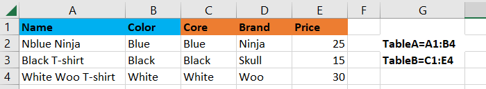
Assume that you have two data sets:
- Table A with columns A and B
- Table B with columns C, D, and E
In Table A, you want to look up the value in column B based on the value in column A.
In Table B, you want to look up the value in column E based on the value in column C.
To perform a VLOOKUP on a VLOOKUP, you will first do a VLOOKUP in Table A to find the value in column D based on the value in column A.
Then, you will use the result from the first VLOOKUP as the lookup value in the second VLOOKUP to find the value in column E.
Here’s the formula:
=VLOOKUP(VLOOKUP(A2, TableA, 2, TRUE), TableB, 3, TRUE)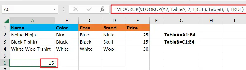
In this example, A2 is the lookup value in Table A, TableA is the data range for Table A, 2 is the column number for column B, TRUE specifies an exact match, TableB is the data range for Table B, and 3 is the column number for column E.
10. How To Use VLOOKUP Function in Excel VBA
The VLOOKUP function can also be used in VBA (Visual Basic for Applications), the programming language for Excel. The syntax for using VLOOKUP in VBA is similar to using it in a formula in a cell.
Here’s an example of how to use VLOOKUP in VBA:
Sub vlookupExample()
'Declare the variables
Dim LookupValue As String
Dim TableArray As Range
Dim ColIndexNum As Integer
Dim RangeLookup As Boolean
'Set the variables
LookupValue = "Black T-shirt"
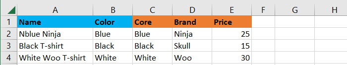
Set TableArray = Worksheets("Sheet1").Range("A1:C4")
ColIndexNum = 2
RangeLookup = False
'Execute the VLOOKUP function
result = Application.WorksheetFunction.VLookup(LookupValue, TableArray, ColIndexNum, RangeLookup)
'Display the result
MsgBox result
End Sub
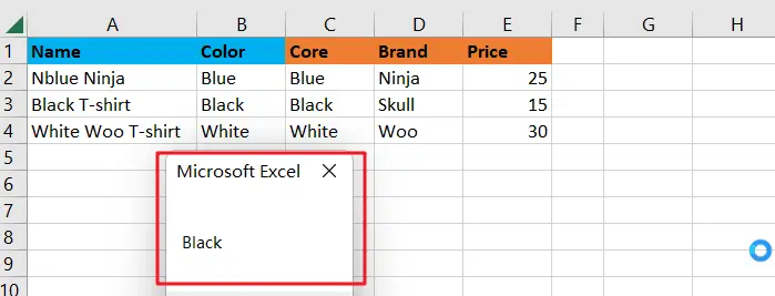
In the above code, the LookupValue is set to “Black T-shirt” and the TableArray is set to the range A1:C4 on a worksheet named “Sheet1“. The ColIndexNum is set to 2, which means the second column of the TableArray will be returned as the result. The RangeLookup argument is set to False, which means an exact match is required.
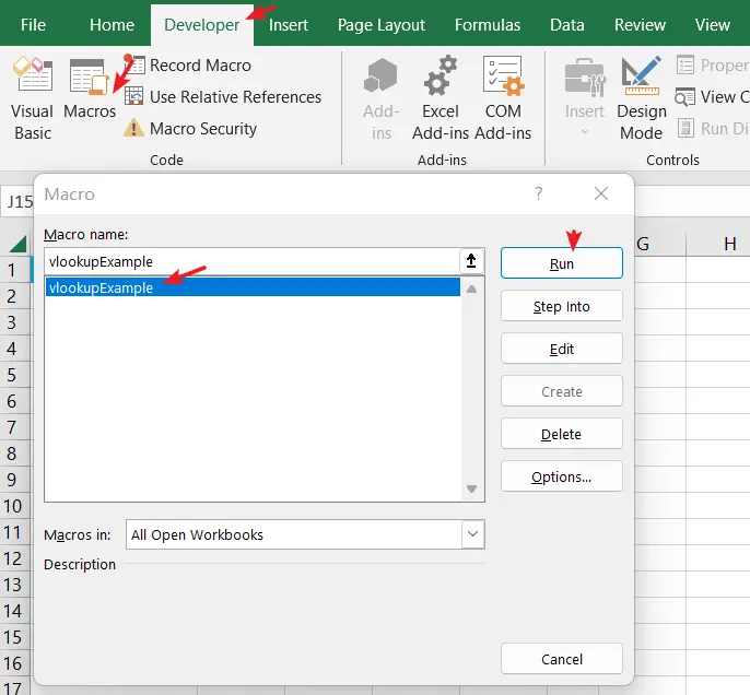
Then You can Click on “Macros” button in Code group, choose “vlookupExample” Macro from “Macro” window, then click “Run” button.
Let’s see the final result as below:
VLOOKUP Function Examples
11. How To Do a VLOOKUP with an IF Function
You can use the IF function (a logical function)in combination with the VLOOKUP function together to return a specified result if the lookup value is not found in the table array.
Suppose you have two tables in Excel, one with a list of product names and their prices (table array), and another with a list of product names (lookup value) and you want to retrieve the corresponding prices, but return a “Not Found” message if the lookup value is not in the table array.
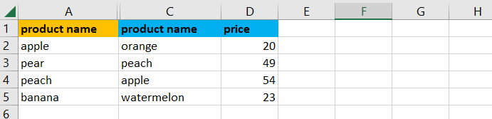
=IF(ISNA(VLOOKUP(A2,$C$2:$D$5,2,FALSE)),"Not Found",VLOOKUP(A2,$C$2:$D$5,2,FALSE))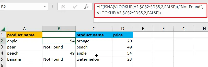
Note:
- The ISNA function checks if the VLOOKUP function returns the #N/A error, meaning the lookup value is not found in the table array.
- If the lookup value is found, the VLOOKUP function returns the corresponding price.
- If the lookup value is not found, the IF function returns the “Not Found” message.
12. How To Use VLOOKUP with AND Function
The “Vlookup” function in Microsoft Excel can be combined with the “And” function to perform a search based on multiple criteria. The syntax for this combined formula is:
=VLOOKUP(lookup_value,table_array,col_index_num, [range_lookup], (And(condition1, condition2, ...)))The above And function checks multiple conditions and returns “TRUE” if all conditions are met, and “FALSE” otherwise.
13. VLOOKUP Function with & Operator
The & operator in Excel is used to concatenate or join together two or more strings. It can be used in combination with the VLOOKUP function to dynamically reference cells or ranges within the formula.
For example, if you have a table in the range A1:C5 and you want to search for a value in column B, you can use the following formula:
=VLOOKUP(A2,A1:C5,2,0)If you want to dynamically reference the range of cells in the table based on the value in a separate cell, you can use the & operator to concatenate the cell reference with the column letter:
=VLOOKUP(A2,A1&":"&C5,2,0)14. VLOOKUP Function with CHOOSE Function
The CHOOSE function in Excel is used to select one item from a list of values based on a specified index number. It can be used in combination with the VLOOKUP function to dynamically choose the column to return a value from, based on the value of a separate cell.
For example, if you have a table in the range A1:C5, and you want to return a value from either column B or column C based on the value of a separate cell (cell D1), you can use the following formula:
=VLOOKUP(A2,A1:C5,CHOOSE(D1,2,3),0)This formula uses the value in cell D1 as the index number for the CHOOSE function, which in turn selects either 2 or 3 as the col_index_num for the VLOOKUP function. If the value in cell D1 is 1, the formula returns a value from column B. If the value in cell D1 is 2, the formula returns a value from column C.
15. VLOOKUP Exact Match
When range_lookup is false, the VLOOKUP formula performs an exact match lookup. It means that only if the lookup value is found in the first column of the data table, the value of the corresponding column is returned, and if the lookup value does not appear in the first column, the error value #N/A is returned.
Example:
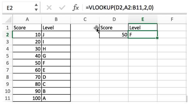
Enter “=VLOOKUP” in E2, enter details of arguments according to the lookup value and the table. In this example, we want to find the correct level for score 50, so 50 is the lookup value. The data table is A2:B11 which records the correspondence between grades and levels. Level is recorded in the second column of data table, so column index number is 2. At last, we want to get an exact match result, so enter “0” or “false” in the last argument.
| Argument | Value |
| lookup_value | D2 |
| table_array | A2:B11 |
| index_num | 2 |
| range_lookup | 0 |
In this example, lookup value appears in the first column of data table. If it doesn’t appear, an error value #N/A will be returned.
16. VLOOKUP Approximate Match
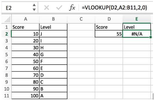
When range_lookup is true, the VLOOKUP function performs an approximate match lookup. Meaning that if the lookup value is not found in the first column of the data table, it returns the value of the corresponding column of the maximum value of all values less than the lookup value. Let’s look at the following example for a concrete analysis.
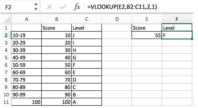
At the end of the previous paragraph “VLOOKUP Exact Match”, we got an ERROR because score “55” does not appear in the first column of the data table. Now let’s change the range_lookup value to 1 (approximate match) and see the difference in the result.
This time level “F” is returned in level value. See the example below:
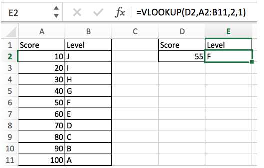
Referring to the rules of the VLOOKUP function, if no lookup value is found, the function will find the value closest to the lookup value. And the closest value should be a value less than the lookup value, and it is also the largest of all values less than the lookup value. In this example, the largest value less than 55 is 50, so VLOOKUP returns the corresponding level to 50.
| Argument | Value |
| lookup_value | D2 |
| table_array | A2:B11 |
| index_num | 2 |
| range_lookup | 1 |
You can also assume that the passing line for an F level is 50 and for an E level is 60, and if you fail to reach 60, you will only be F.
17. VLOOKUP with Absolute Range Reference
We know that in the Excel workbook, enter a formula in a cell, if the formula is dragged to other cells, cell references or range references used in the formula arguments will be automatically updated, so that we can directly drag and drop the formula into other cells to copy the formula without having to manually update the arguments.
See example below:
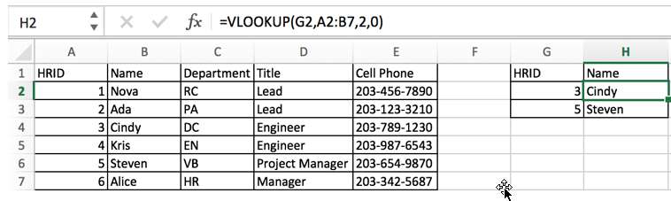
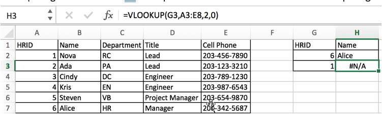
In this case, we have entered a VLOOKUP formula in H2, and we can drag the formula directly to H3 to reuse the formula, while the lookup value and lookup range get updated due to moving the formula. The VLOOKUP formula is dragged down from H2 to H3, the lookup value is updated from G2 to G3 and lookup range is updated from A2:B7 to A3:B8 accordingly.
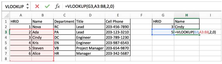
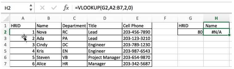
In this example, along with the movement of the formula, the lookup value HRID=5 still appears in the first column even though the lookup range has been moved down one row, and we can get the correct employee name by this formula. However, in some cases, this considerate automatic update can cause errors in real cases, see the following example.
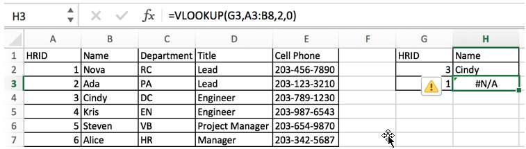
In this case, HRID=1 does not appear in the first column of data table A3:B8, so the lookup value does not exist and the formula returns error #N/A. In fact, in most VLOOKUP formulas, if the lookup range is fixed, we should lock the range by adding $ in front of the index numbers of the rows and columns, so that no matter where we copy this formula to later, the locked range will not be changed.
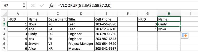
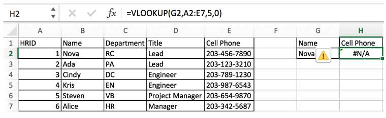
Add $ before row and column indexes to lock both row and column. The lookup range is $A$2:$E$7. Even copy this formula to H3, the range is still $A$2:$E$7.
Sometimes we just need to lock the row or column by adding $ before the index number of the row or column, so that the locked row or column will not be changed by the movement of the formula. For more examples you can refer to the section “VLOOKUP returns multiple column values”.
18. VLOOKUP with Duplicate Lookup Value
VLOOKUP has an important feature, when looking for duplicate values, the first duplicate value will be matched by default.
Look at the following example. There are two “Cindy” in the second column. When we use VLOOKUP to find the cell phone number corresponding to “Cindy”, the phone number of the first Cindy will be returned.
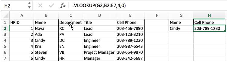
We can add more helper information to return unique matching values. For more details and explanations, you can refer to the section “VLOOKUP Two-conditional Lookup”.
19. VLOOKUP Lookup the Largest/Smallest value
Based on the property that when VLOOKUP encounters a duplicate lookup value, it only returns the value that matches the first lookup value, we can use VLOOKUP function to find the maximum or minimum value of the data. First of all, we need to sort the results of the column.
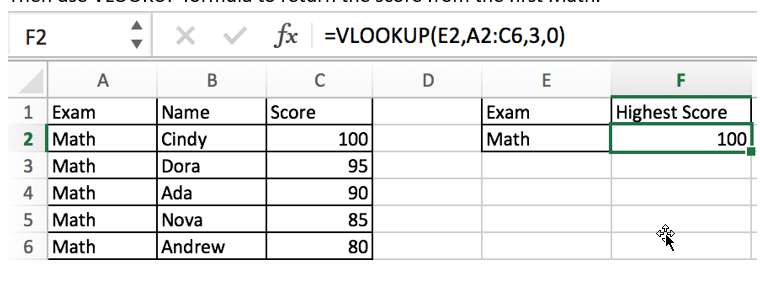
See the example below. Fill in the highest score in the exam.
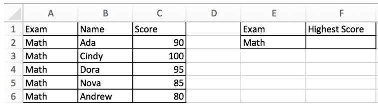
Sort the results in descending order. Check on “Expand the selection” when soring result column, so that sorting will be applied to all three columns.
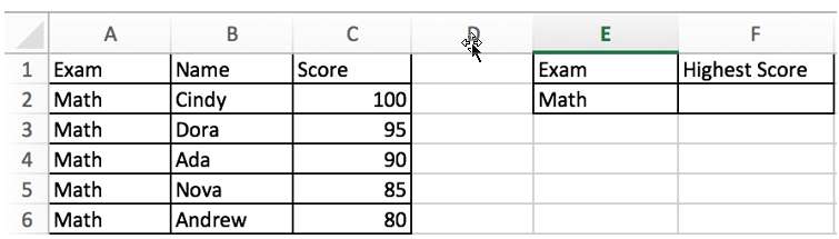
Then use VLOOKUP formula to return the score from the first Math.
20. VLOOKUP Reverse Lookup
Refer to above example we can see that VLOOKUP can only find data to the left of the lookup value in the data table. If you want to find the data to the right of the lookup value, it is called a reverse lookup. A reverse lookup needs the help of IF function.
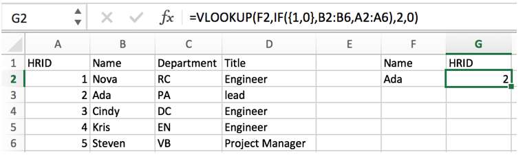
The above example is a very typical example, usually we find the name by looking up the HRID, this is finding the HRID by name.
In the formula, the table_array is a IF formula, IF({1,0},B2:B6,A2:A6) will create a new two-column lookup table with the name first and the HRID second. This allows us to do reverse lookups.
| Argument | Value |
| lookup_value | F2 |
| table_array | IF({1,0},B2:B6,A2:A6) |
| index_num | 2 |
| range_lookup | 0 |
21. VLOOKUP to Return Multiple Values
A one-to-many lookup returns multiple results by looking for a unique lookup value. VLOOKUP can implement a one-to-many lookup with the help of creating a helper column.
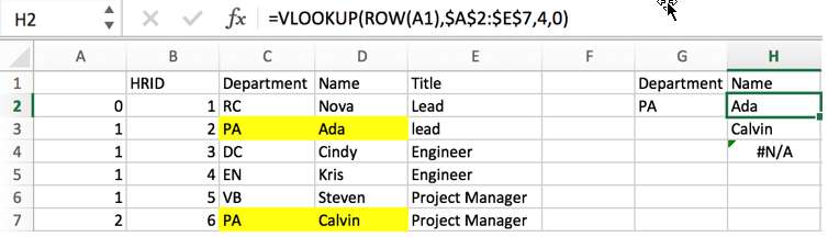
In this example, it is clear that there are two people in our table who belong to department “PA”. If we use the normal VLOOKUP formula “=VLOOKUP(G2,B2:E7,3,0)” to return the matching people in department “PA”, only one value “Ada” will be returned, because VLOOKUP will stop searching when it encounters the first “PA” in the data table.
To output all values corresponding to the lookup value, we need to create a new helper column. See details in below steps.
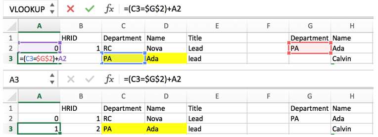
Step 1: First we insert a blank column on the left side of the data table, then enter =(C2=$G$2)+A1 in cell A2. Here A1 is 0, C2=$G$2 is a logical test, if it is true, it returns value 1, and if it is false, it returns value 0. In A2, the logical test is false, so the result is equal to “0+0=0”.
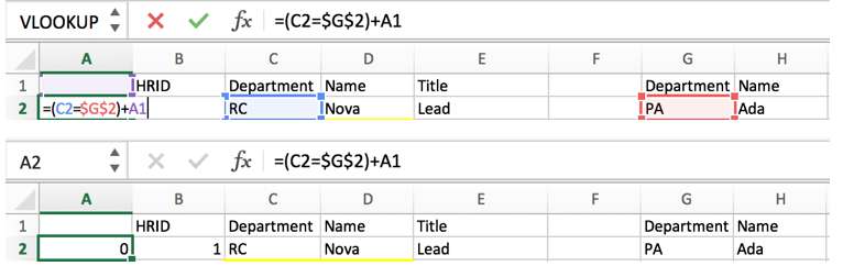
Step 2: Drag the handle down to copy the formula to A3:A7, so that for every PA department encountered, it will be increased by 1.
Step 3:In H2 enter the formula:
=VLOOKUP(ROW(A1),$A$2:$E$7,4,0).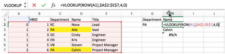
In this formula, the lookup value is ROW (A1). ROW (A1) returns the cell reference A1’s row index number, which returns a value of 1. In fact, in the helper column, the first number “1” and the number “2” both correspond to the PA department (because the counter only increases by 1 when it encounters PA), what we want to do is to query the first two numbers “1” and “2”, so here we need the help of the Excel ROW function.
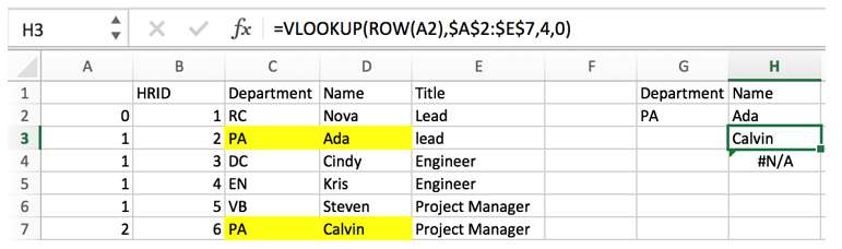
Step 4:Drag the handle down to fill out the form below. You can stop filling out the form when an error value appears, which means the search is complete.
22. VLOOKUP to Return Multiple Column Values
When we want to return multiple columns of data based on the lookup value, we can enter the VLOOKUP function once in each column. Although this can also be effective, it is not a quick way to do it.
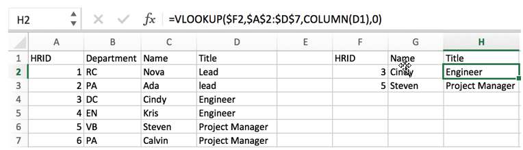
Please see the following example. We want to know the “Name” and “Title” information based on the HRID provided. Although we can enter two VLOOKUP formulas with different column index numbers, this approach is not convenient if we want to get multiple column values from the original data table.
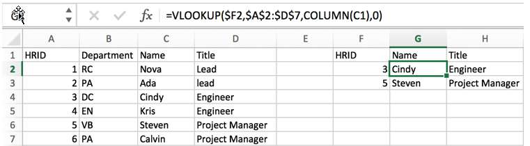
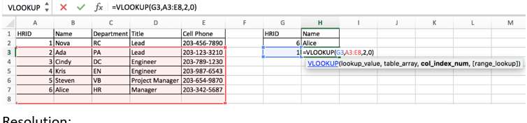
In above screenshot, you can see that we build the following VLOOKUP formula:
=VLOOKUP($F2,$A$2:$D$7,COLUMN(C1),0)Using this formula, we can drag the handle directly down to fill the “Name” and “Title” information in the form we want (G2:H3).
The steps are as follows:
Step 1: In cell G2 enter the formula =VLOOKUP().
Step 2: Enter cell $F2 in the lookup value and lock column F with ($) because the horizontal fill needs to keep column F unchanged. This step ensures that if you drag this formula to fill H2, column F remains unchanged and the lookup value remains $F2 (the column is locked, the row remains unchanged).
Step 3: Enter $A$2:$D$7 in table_array. Add ($) in front of the column and row indexes to lock this range. Therefore, this range remains the same no matter where the user copies the formula.
Step 4: Enter COLUMN(C1) in col_index_num. COLUMN(C1) returns cell C1’s column number, which returns a value of 3. If drag this formula to H2, COLUMN(C1) is changed to COLUMN(D1), which returns a value of 4, so that VLOOKUP will returns a value in the fourth column of data table. The fourth column is “Title”.
Step 5: Enter “0” in range_lookup to perform an exact match.
Step 6: Drag the handle down to fill the form G2:H3.
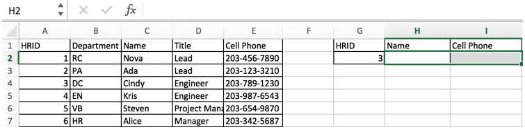
There is another way to return multiple column values for multiple items at the same time based on the same lookup value.
See the following example.
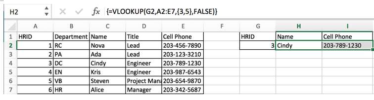
Step1: Select range H2:I2.
Step2: In the formula bar enter the VLOOKUP formula =VLOOKUP(G2,A2:E7,{3,5},FALSE).
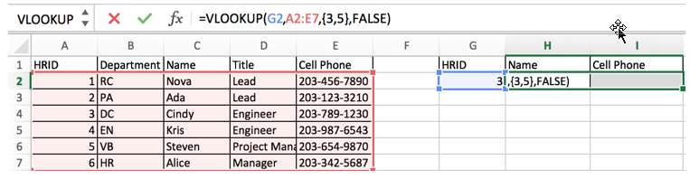
Please refer to the third argument col_index_num, different from usual, we only enter one column number in this argument, this time we enter an array containing two column numbers, so in step #1 we choose the range H2:I2 (one row and two columns) to save the returned result.
Step3: As this is an array formula, press Control+Shift+Enter to load result.
23. VLOOKUP Two-Conditional Lookup
This situation applies to tables with duplicate lookup values, because the lookup value is not unique and VLOOKUP may get the wrong result, so we need to add a condition as the lookup value.
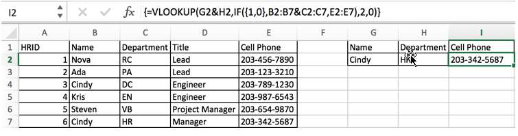
See the following example. There are two conditions “PA” and “Lead”. “PA” and “Lead” are both duplicate in the table. We need to get correct person’s name based on the two conditions.
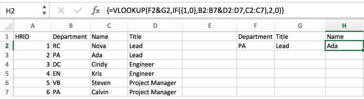
In this example, the formula is :
=VLOOKUP(F2&G2,IF({1,0},B2:B7&D2:D7,C2:C7),2,0).To solve this problem, we can combine the two conditions “PA” and “Lead” into “PALead” and combine the content in the “Department” column and “Title” column into one column, then we can lookup “PALead” in this column.
In addition to the new column, we should also add the “Name” column (where we want to get the values) to the right of the new column. This will give us a new table with two columns, the first with the “Department” and “Title”, and the second with “Name”.
To create this new data table, we need the help of Excel’s IF function. The formula IF({1,0},B2:B7&D2:D7,C2:C7) can create a table according to our requirements.
IF({1,0},B2:B7&D2:D7,C2:C7) returns the following array:
{"RCLead","Nova";"PALead","Ada";"DCEngineer","Cindy";"ENEngineer","Kris";"VBProject Manager","Steven";"PAProject Manager","Calvin"}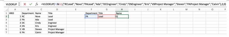
In this example, we enter F2&G2 in lookup value. We concentrate F2 and G2 to get a new condition “PALead”.
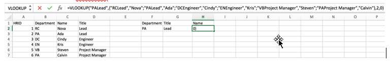
After completing above steps, enter “2” in col_index_num to return a value in “Name” column, and enter “0” in range_lookup to perform an exact match. As this is an array formula, so we should press “Control+Shift+Enter” to get a value.
24. VLOOKUP with Wildcards
VLOOKUP can perform the search function normally if the lookup value contains wildcards. A wildcard is a special statement containing mainly asterisk (*) and question mark (?), wildcards are often used to fuzzy search for files. It can be used in place of one or more real characters when searching for a folder; wildcards are often used in place of one or more real characters when the real characters are not known or when you are too lazy to type the full name.
- (*) – An asterisk stands for one or more characters
- (?) – A question mark stands for single one character
See the example below.
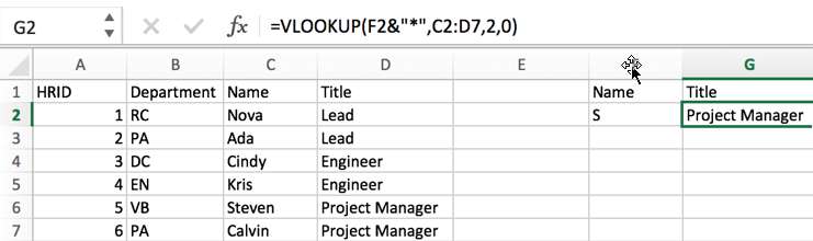
In this example, only one letter “S” is shown in cell F2. We cannot look up this letter in the “Name” list because the spelling of the name is incomplete. We can determine that the first character inside the name is “S”. If we want to find a suitable title for this person, we can set the lookup value to F2&”*”, and the symbol (&) will combine the letter “S” in cell F2 with the wildcard character (*), so the lookup value is “S*”.
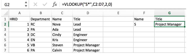
“S*” represents a string that starts with the letter “S”. Therefore, when searching the list of names, “Steven” will be locked and the corresponding value “Project Manager” will be returned.
25. VLOOKUP Range Lookup by Approximate Match
A range lookup is a range that corresponds to a result, such as a grade based on a range of scores like “50 to 60”. In order to perform a range lookup, we need to use the VLOOKUP approximate match function.
First we need to make sure that the first column of the table is sorted in ascending order. The lookup value must fall in one of the data ranges in the first column.
We then use VLOOKUP to do a regular lookup, where we need to set the fourth parameter to 1, which means that VLOOKUP performs an approximate match.
The following example is copied from “VLOOKUP Approximate Match”. We have added a column in front of the original table to explain the individual score segments. You can refer to “VLOOKUP Approximate Matching” for more details.
You just need to remember that when VLOOKUP performs an approximate match, VLOOKUP will take the value which is the largest value among all values less than the actual lookup value as the lookup value.
VLOOKUP Error Value Handling
26. VLOOKUP returns error #N/A
Failure reason 1:
The lookup value doesn’t appear in the lookup range.
Resolution:
Check lookup value and make sure it lists in the first column of data table.
Failure reason 2:
The lookup value doesn’t list in the first column.
Resolution:
Check lookup value and make sure it lists in the first column of data table.
Failure reason 3:
Lookup range is not locked. So lookup value cannot be found in moved lookup range.
Resolution:
Add $ to lock lookup range. Make sure lookup value exists in the first column of data table.
27. VLOOKUP returns error #REF!
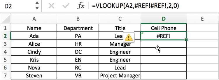
Failure reason 1:
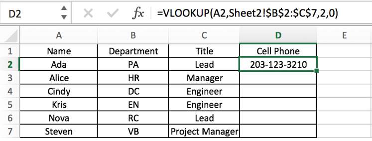
The lookup range cannot be found. For example, delete Sheet2, which holds the lookup range, so the range reference cannot be found.
Sheet2 is not deleted.
Sheet2 is deleted.
Resolution:
Check lookup range to ensure values are saved in the entered range reference.
Failure reason 2:
If the number of columns entered in the third argument is greater than the actual number of columns in the second argument lookup range.
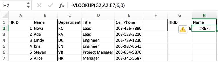
Resolution:
Check the third argument “col_index_num”.
28. VLOOKUP returns error #VALUE
Failure reason 1:
If the argument “col_index_num” contains text or is less than 0, then error #VALUE is returned. Normally, we do not accidentally write a negative value or text to a column index, but if the column index is a value passed by another formula, it is possible to generate this error.
Resolution:
Check the third argument “col_index_num”.
29. VLOOKUP returns error #NAME
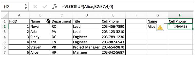
Failure reason 1:
The lookup value format is incorrect.
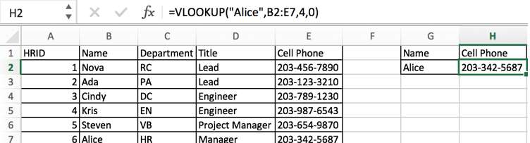
“Alice” is a text, if we enter “Alice” in the lookup value, rather than using the cell reference G2, the text or string should be quoted in double quotes, as shown below.
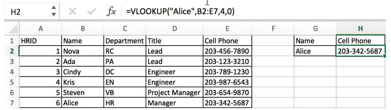
Resolution:
Check format for all arguments.
30. VLOOKUP Eliminate the Error Value/ No Error Value Returned by VLOOKUP
In VLOOKUP formulas, if you cannot find the lookup value in the provided data table, then the formula will return an error value such as #N/A, which doesn’t seem appropriate because displaying the error in the table will make the table look unprofessional. So, how to eliminate this error value or make it show 0 or empty when it returns and detects an error, we will show you a convenient way to eliminate the error.
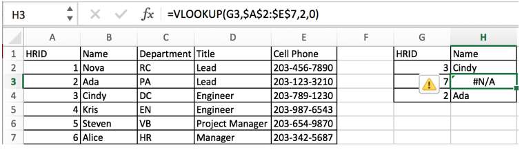
The VLOOKUP formula returns an error because HRID “7” doesn’t appear in the first column. To convert the error value to empty or “0” value, we can add the IFERROR function in front of the VLOOKUP function.
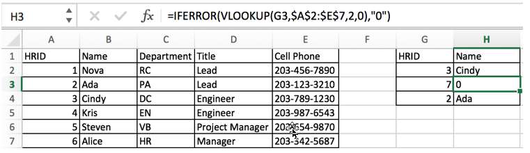
Use formula =IFERROR(VLOOKUP(G3,$A$2:$E$7,2,0),”0″) to set error value to “0”.
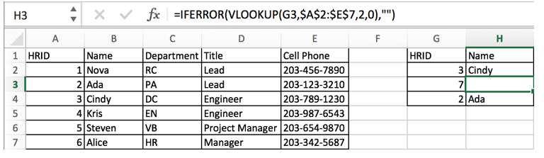
Use formula =IFERROR(VLOOKUP(G3,$A$2:$E$7,2,0),””) to set error value to empty.
See Also: