Sometimes we may meet the case that to sum numbers with the pre-condition “less than X”. We only want to sum numbers which are less than a supplied number. In this article, we will show you the method to resolve this problem by formulas with the help of Excel SUMIF and SUMIFS functions.
Through a simple instance below, we will introduce you the syntax, argument and the usage of SUMIF and SUMIFS functions. We will let you know how the formula works step by step to reach your goal clearly. After reading the article, you may have a simple understanding of SUMIF/SUMIFS functions.
EXAMPLE
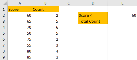
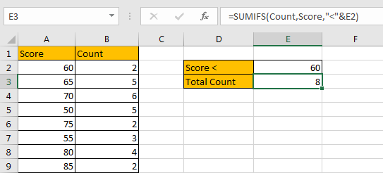
Refer to the left-hand table, we can see that there are two columns “Score” and “Count”. For each score, its adjacent cell records the number “how many students get this score”. In the right-hand table, it is a simple summary table. There is only one condition that “score: less than 60”, and our expectation is counting the total number of students whose score is less than 60. In this case, user can enter any value into E2, it is a dynamic value. In the formula, we just use cell reference E2 to represent the value, so, if E2 value is changed, the returned value is also changed accordingly.
As we want to sum numbers from “Count” column based on the criteria “Score < 60 (value in E2)”. We need to find out all scores that meet our requirement, and then sum up values in “Count” column accordingly. To resolve this issue by formula, we can apply Excel SUMIF or SUMIFS functions.
FORMULA 1 – APPLY SUMIF FUNCTION
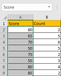
Step 1: Select A2:A9, then in Name Box define a name for this range, just use the column header ‘Score’.
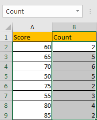
Step 2: Select B2:B9, in Name Box define a name for this range, for example ‘Count’.
Note: Above two steps are not required, they are optional, you can directly use cell or range reference like A2:A9, B2:B9 in your formula, but for understanding well, we name ranges in advance.
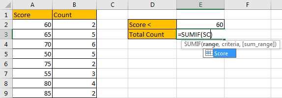
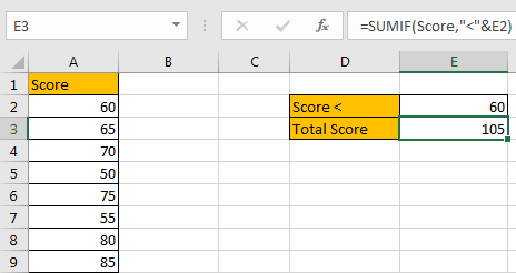
Step 3: In E3, enter the formula =SUMIF(Score,”<“&E2,Count).
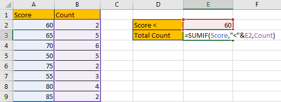
Note: In step#1 and step#2 we already name ranges “Score” and “Count”, so when entering the range information into formula, just after typing “Sc…”, our named range “Score” is loaded, just select it from dropdown list. As we explained in step#2, you can also hold and drag A2:A9 to fill the argument as well.
Step 4: Press Enter after typing the formula.
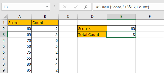
In column A, cell A5 (50), A7 (55) are less than 60, the corresponding counts are 5 (in cell B5), 3 (in cell B7), so the total count is 5+3=8. The formula works correctly.
SUMIF FUNCTION INTRODUCTION
SUMIF function can be seen as SUM+IF, it sums numbers based on criteria. it allows user provides one pair of ‘criteria range’ and ‘criteria’.
For SUMIF function, the syntax is:
SUMIF(range, criteria, [sum_range]) – if sum range=range, then sum range can be omitted.
SUMIF function allows wildcards like asterisk ‘*’ and question mark ‘?’, it also allows logical operators within its argument. If wildcards or logical operators are required, they should be enclosed into double quotes (““).
SUMIF ARGUMENTS EXPLAINATION
SUMIF – RANGE
We need to compare each score in “Score” column with 60, so “A2:A9” is the ‘range’.
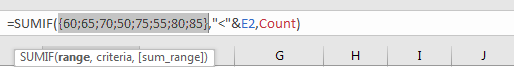
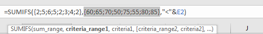
In the formula bar, select “Score”, press F9, all values in “Score” are listed in an array.
SUMIF – CRITERIA
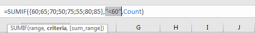
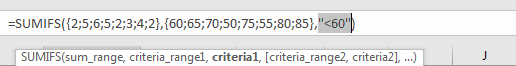
We enter “<”&E2 as “criteria”. If logical operator is used, it should be quote within double quotes “”; In E2, we enter “60” to filter scores; to concentrate logical operator “<” and number “60”, we need to use a special character “&” to connect them, if “&” is missing, formula quits typing directly.
In the formula bar, select the completed criteria, press F9.
SUMIF – SUM RANGE
In this instance, we need to count numbers of student whose score is less than 60. So, cell reference “B2:B9” in “Count” column is the ‘sum range’.
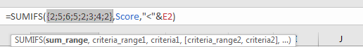
In the formula bar, select “Count”, press F9, all values in “Count” are listed in an array.
SUMIF WORKFLOW
After explaining each argument in the formula, now we will show you how the formula works with the help of these arguments.
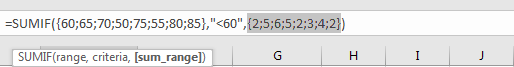
=SUMIF({60;65;70;50;75;55;80;85},”<60″,{2;5;6;5;2;3;4;2})
We have a pair of range and criteria:
RANGE: {60;65;70;50;75;55;80;85}
CRITERIA: “<60”
Compare each number in the array with 60; if number satisfies the condition “<60”, mark it in bold:
{60;65;70;50;75;55;80;85} – In bold if it is <60
As bold number meets our requirement, so record a ‘True’ for them in the array; otherwise, record a ‘False’ for others.
{Flase;False;False;True;False;True;False;False}
Convert ‘True’ to ‘1’ and ‘False’ to ‘0’ to make this array can be taken into calculation in next step.
{0;0;0;1;0;1;0;0}
Now, we have below two arrays:
{2;5;6;5;2;3;4;2} – Sum Range
{0;0;0;1;0;1;0;0} – from above steps we know that if number is less than 70, 1 is displayed in this number’s position
We list the two arrays in two rows, in the same column multiply the two numbers, and save their product in another row.
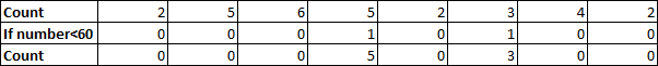
Sum up all numbers in the third row. You can use SUM function here and select all values in the third row as reference.
5+3=8
NOTE
If there is no “Count” column, and only “Score” column exists, and you want to sum numbers with the condition “number is less than 60”, you can also use SUMIF function here. In this situation, the sum range and criteria range are the same as there is only one range reference A2:A9, so, the last argument ‘sum range’ can be omitted in the formula.
FORMULA 2 – APPLY SUMIFS FUNCTION
Now, let’s try to apply SUMIFS function to resolve this issue. The first two steps are the same.
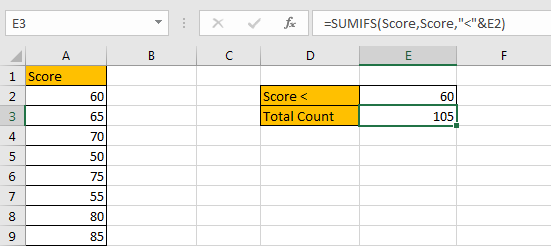
Step 3: In E3, enter the formula =SUMIFS(Count,Score,”<“&E2).
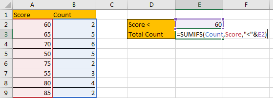
Note: We can see in SUMIFS formula, we use the same parameters compare with SUMIF, the difference is “Count” is moved to the first position.
Step 4: Press Enter after typing the formula.
SUMIFS FUNCTION INTRODUCTION
SUMIFS function can be seen as SUM+IFS, it allows user provides multiple ‘criteria range’ and ‘criteria’ combinations.
For SUMIFS function, the syntax is:
SUMIFS(sum_range, criteria_range1, criteria1, [criteria_range2, criteria2], …).
SUMIFS function allows wildcards like asterisk ‘*’ and question mark ‘?’, it also allows logical operators within its argument. If wildcards or logical operators are required, they should be enclosed into double quotes (““).
SUMIFS ARGUMENTS EXPLAINATION
SUMIFS and SUMIF share the same parameters in this instance.
SUMIFS – SUM RANGE
SUMIFS – CRITERIA RANGE
SUMIFS – CRITERIA
SUMIFS WORKFLOW
SUMIFS and SUMIF have the same criteria range, criteria and sum range, they are processed with the same steps exactly.
NOTE
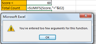
Unlike SUMIF function, if sum range and criteria range are the same in a formula, sum range is still required.
Warning message pops up if missing argument.
SUMMARY
1. SUMIFS function can handle multiple pairs of criteria ranges and criteria. Sum range is the first argument among all arguments.
2. SUMIF function can handle one pair of criteria range and criteria. Sum range is the last argument among all arguments.
3. They allow user defined range name, wildcards, logical operators.
Related Functions
- Excel SUMIFS Function
The Excel SUMIFS function sum the numbers in the range of cells that meet a single or multiple criteria that you specify. The syntax of the SUMIFS function is as below:=SUMIFS (sum_range, criteria_range1, criteria1, [criteria_range2, criteria2], …)… - Excel SUMIF Function
The Excel SUMIF function sum the numbers in the range of cells that meet a single criteria that you specify. The syntax of the SUMIF function is as below:=SUMIF (range, criteria, [sum_range])…