Sometimes for data listed in rows, we may want to sum data every Nth column, for example sum data only in ODD column or EVEN column (every 2 column). In our daily life, we may meet many cases like this. It is necessary for us to have the knowledge of sum data by every Nth column in excel. Actually, excel built-in functions SUMPRODUCT, MOD, and COLUMN can help us resolve this issue properly.
This article will show you ‘to sum every Nth column’ based on SUMPRODUCT, MOD and COLUMN functions. MOD function is frequently used in sum every Nth case, COLUMN returns column number for a reference. Thus, SUMPRODUCT function is used for ‘sum’, the combination of MOD and COLUMN works on locate ‘every Nth column’. We will introduce above three functions with simple examples, descriptions, screenshots and explanations in this article, and also show you the usage of them. Finally, we will let you know the formula workflow step by step clearly.
After reading the following article, I’m sure you can have a simple understanding of SUMPRODUCT, MOD and COLUMN functions. Besides, you can learn well on sum data every Nth column/row. I’m sure you can work well with these functions in your daily work in the future.
EXAMPLE:
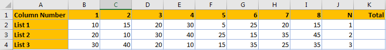
We prepare three lists and set ‘N’ value in J column. N means to sum data every ‘Nth’ column. For example, for list2, N=2, so we sum data every 2 column, in fact we need to sum data in C3, E3, G3 and I3. As N is not a fixed value, it can be any integer, so we need to take this into consideration when creating a formula.
FORMULA:
To figure out this problem, we can apply a formula based on SUMPRODUCT, MOD and COLUMN functions.
Step 1: In K2 enter the formula =SUMPRODUCT(–(MOD(COLUMN(B2:I2)-COLUMN(B2)+1,J2)=0),B2:I2).

Step 2: Click Enter to get return value. Verify that 140 is calculated correctly.
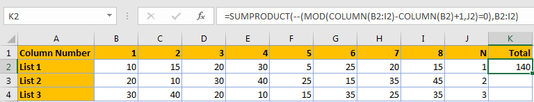
(In list1, N=1, sum data every 1 column means sum data in all columns, we can also use SUM(B2:I2) to sum total directly.)
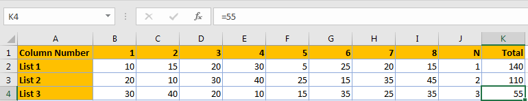
Step 3: Copy the formula to K3 and K4. References are automatically updated in the formula.
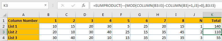
We can see that total values are calculated correctly.
Table of Contents
USAGE OF COLUMN and MOD FUNCTIONS
We have introduced SUMPRODUCT function usage in previous articles. In this formula, the core part is the combination of MOD and COLUMN functions. We will have a brief review about SUMPRODUCT function when analyzing the workflow of each function in the formula.
The Usage of COLUMN Function
For COLUMN function, the syntax as below:
=COLUMN ([reference])
COLUMN function can return the column number for a reference. The reference can be a cell or a range.
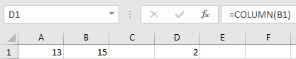
Usage 1: For example, when we enter ‘=column(B1)’ in D1, column number 2 is returned as B column is the second column in this worksheet. Thus, we can see that COLUMN function only returns the column number for the reference (B1 for example) and it is not affected by the reference value (15 in B1).
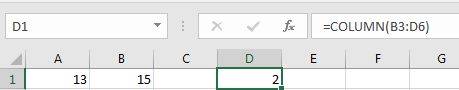
Usage 2: If the reference is a range, COLUMN function will return the column number of the leftmost column when pressing Enter directly after entering the formula. See example below. In this case B3:D6 contains 4 rows and 3 columns, COLUMN function will return the leftmost column (B column in this case), so 2 is returned.
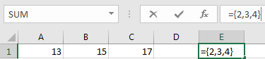
Usage 3: But if the reference is a range, COLUMN function will return a horizontal array contains all column numbers in this range when selecting output part and pressing CTRL+SHIFT+ENTER. See example below. Enter =COLUMN(B3:D6) in E1, then in formula bar press F9, we can get an array {2,3,4}. So in this case, COLUMN function can return an array instead of an integer.
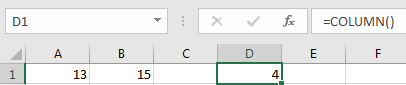
Usage 4: By the way, If the reference is omitted, COLUMN function returns current column number. See example below:
The Usage of MOD Function
For MOD function, the syntax as below:
=MOD(number, divisor)
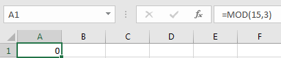
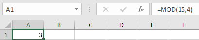
MOD function can return the remainder of the two arguments ‘number is divided by divisor’. We can directly enter the two arguments number and divisor into formula to get remainder, see example below:
Remainder is 0. 0 is returned as 15 is divisible by 3, remainder is 0.
Remainder is not 0. 3 is returned because when dividing 15 by 4, it doesn’t return a whole number, the remainder is 3.
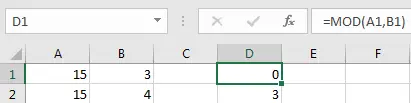
The two arguments also can be two references. Then MOD function will use the reference to execute formula. See example below:
In our instance =SUMPRODUCT(–(MOD(COLUMN(B3:I3)-COLUMN(B3)+1,J3)=0),B3:I3), ‘Number’ is a formula COLUMN(B3:I3)-COLUMN(B3)+1, ‘Divisor’ is a reference J3.
HOW THIS FORMULA WORKS:
After introducing above basic syntax, arguments, usage of COLUMN and MOD functions, we will analysis the working process of our formula in this article. Firstly, we will introduce each function workflow based on list1 and the formula in K2. In our instance list1, for snippet (MOD(COLUMN(B2:I2)-COLUMN(B2)+1,J2)=0), refer to COLUMN function usage#3, COLUMN(B2:I2) actually returns an array {2,3,4,5,6,7,8,9}, please see screenshot below. (select COLUMN(B2:I2) in formula bar, then press F9, you can see the array.)
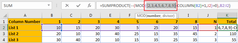
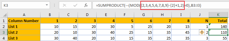
As COLUMN(B2)=2, J2=1, so MOD(COLUMN(B2:I2)-COLUMN(B2)+1,J2) equals to MOD({2,3,4,5,6,7,8,9}-{2}+1,1). Please see screenshot below.
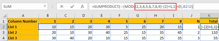
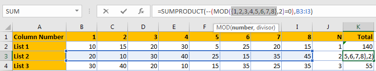
Continue to calculate the formula, we can get MOD({1,2,3,4,5,6,7,8},1).
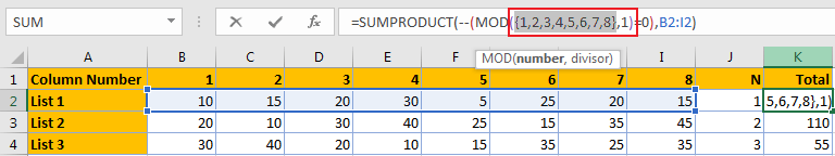
In this formula, array {1,2,3,4,5,6,7,8} is argument ‘Number’, 1 is argument ‘Divisor’, as all numbers in the array are divisible by 1, so MOD({1,2,3,4,5,6,7,8},1)=0 equals to MOD({1,2,3,4,5,6,7,8})=0, compare each value in the array with 0, we can get below result.
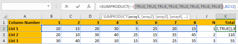
Add double negative symbol (–) before TURE (or FALSE) result to convert TRUE to 1 and FALSE to 0, then the array converts to {1,1,1,1,1,1,1,1}, see screenshot below:
In list1, we can see that as value in J2 is 1, so sum data every 1 column is equivalent to sum all data in list B2:I2. But for list2, we need to sum data every second column, so actually we need to sum data in C3,E3,G3 and I3. Similar to list1, firstly we get all returned values of COLUMN function.
Now number argument is {1,2,3,4,5,6,7,8}, divisor is 2.
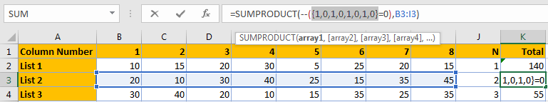
A number is divided by 2, the remainder is 0 or 1. After calculating MOD({1,2,3,4,5,6,7,8},2), we get an array {1,0,1,0,1,0,1,0}.
After comparing with 0, we can get TRUE or FLASE as result.
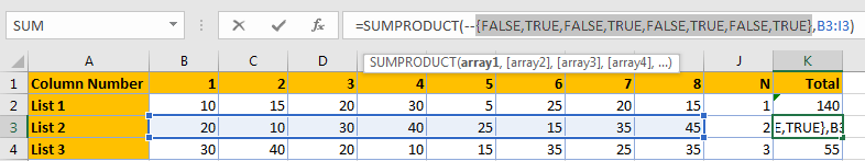
Convert TRUE to 1 and FALSE to 0 by adding double negative (–).
Now we come to the outermost function SUMPRODUCT. SUMPRODUCT function syntax has the following arguments:
=SUMPRODUCT(array1, [array2], [array3], …)
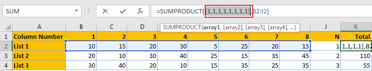
For list1, the last step is =SUMPRODUCT({1,1,1,1,1,1,1,1},B2:I2). We can see that there are two arrays, the first array is {1,1,1,1,1,1,1,1}, the second array is the values in B2:I2 {10,15,20,30,5,25,20,15}.
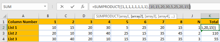
So, SUMPRODUCT({1,1,1,1,1,1,1,1},{10,15,20,30,5,25,20,15}) can be seen as value in one array multiplies by the corresponding value in another array, in this case the final array is equivalent to {1*10, 1*15,1*20,1*30,1*5,1*25,1*20,1*15}={10,15,20,30,5,25,20,15}, then sum data in the array {10,15,20,30,5,25,20,15}, 10+15+20+30+5+25+20+15=140.
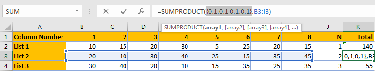
For list2, the last step is =SUMPRODUCT({0,1,0,1,0,1,0,1},B3:I3). We can see that there are two arrays, the first array is {0,1,0,1,0,1,0,1}, the second array is the values in B3:I3 {20,10,30,40,25,15,35,45}.
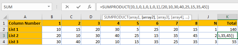
So, for SUMPRODUCT({0,1,0,1,0,1,0,1},{20,10,30,40,25,15,35,45}), multiply value in array1 by the value in array2, so we get {0*20,1*10,0*30,1*40,0*25,1*15,0*35,1*45}={0,10,0,40,0,15,0,45}. SUMPRODUCT({0,10,0,40,0,15,0,45})=10+40+15+45=110.
RESULT:
Let’s check the formula workflow in F3. Actually, the workflow for list3 is the same, only divisor is changed to 3 for MOD part.
Step 1: Execute COLUMN function, convert all reference to real values.
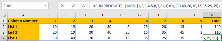
Step 2: Execute MOD function.
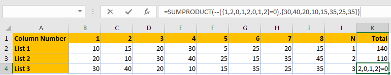
Step 3: Compare values with 0 and convert TRUE/FALSE to 1/0.
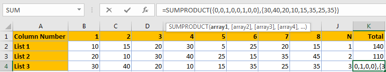
Step 4: Execute SUMPRODUCT function, to sum data based on two arrays. SUMPRODUCT({0,0,20,0,0,35,0,0}=55. So we get 55 in K4.
SUMMARY:
- COLUMN function returns an array if COLUMN function is entered as a horizontal array formula.
- COLUMN function returns the leftmost column if COLUMN function is not entered as a horizontal array formula.
- MOD function is often used in calculating ‘Nth’ rows/columns cases.
- To sum ODD columns:
=SUMPRODUCT(–(MOD(COLUMN(list)-COLUMN(first cell)+1,2)=1),list)
- To sum EVEN columns:
=SUMPRODUCT(–(MOD(COLUMN(list)-COLUMN(first cell)+1,2)=0),list)
Related Functions
- Excel SUMPRODUCT function
The Excel SUMPRODUCT function multiplies corresponding components in the given one or more arrays or ranges, and returns the sum of those products. The syntax of the SUMPRODUCT function is as below:= SUMPRODUCT (array1,[array2],…)… - Excel MOD function
he Excel MOD function returns the remainder of two numbers after division. So you can use the MOD function to get the remainder after a number is divided by a divisor in Excel. The syntax of the MOD function is as below:=MOD (number, divisor)…. - Excel COLUMN function
The Excel COLUMN function returns the first column number of the given cell reference.The syntax of the COLUMN function is as below:=COLUMN ([reference])….